Prescribed displacement of a unit cube
1 Objective
Verify zero and nonzero prescribed displacement boundary conditions applied independently to the six faces of an immersed unit cube. The study checks the resulting displacement field with face-based multi-point probes and directly from the generated surface-element sets in the Abaqus output database. It also checks the constant stress field on a three-dimensional interior probe grid.
2 Geometry
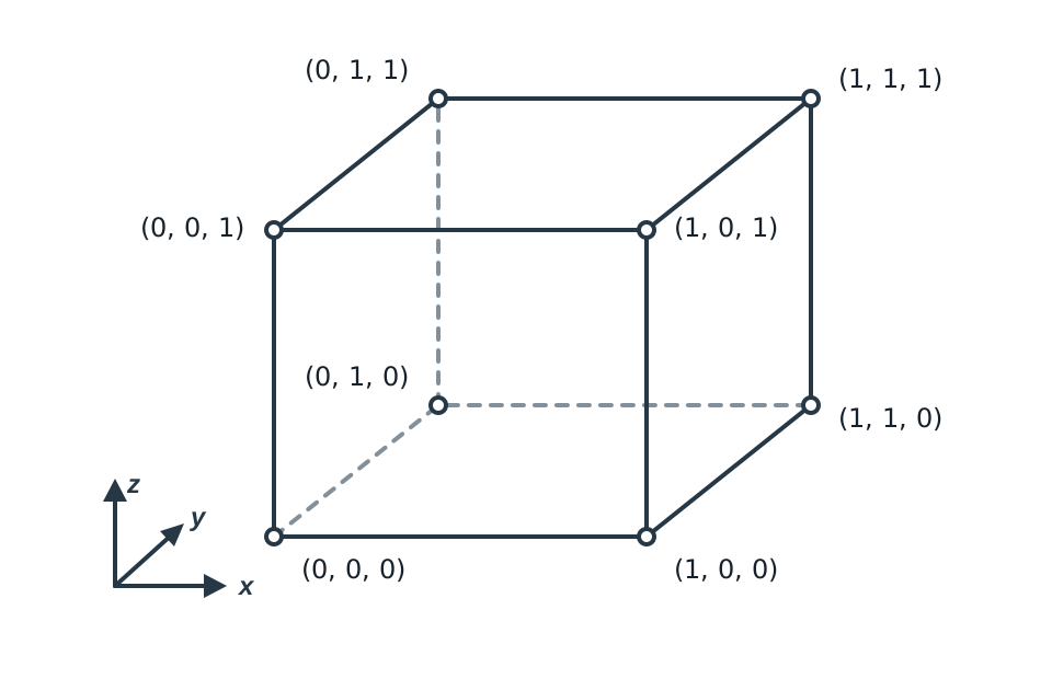
The geometry occupies
\[ x\in[0,1],\qquad y\in[0,1],\qquad z\in[0,1]. \]
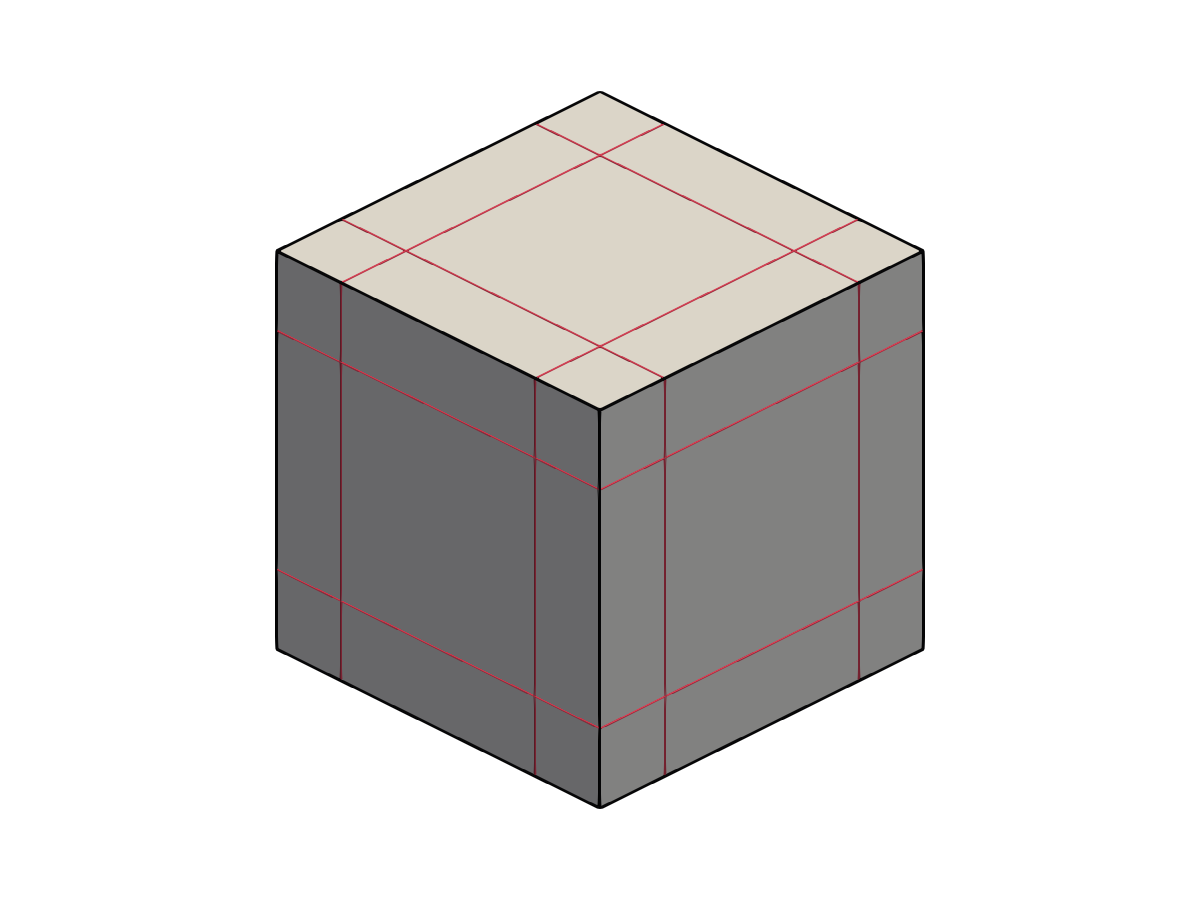
The cube is embedded in an axis-aligned rectilinear background grid (Figure 1). The spline grid is generated independently of an Abaqus finite-element mesh, and all six cube faces trim the background discretization.
3 Material
The cube is homogeneous and isotropic with the small-strain, linear-elastic properties in Table 1. The Abaqus material definition uses isotropic linear elasticity, specified by Young’s modulus and Poisson’s ratio, as defined under Linear Elastic Behavior in the Abaqus Materials Guide [1]. In the generated input deck this is the *ELASTIC option. Its Abaqus Keywords Guide entry confirms that an omitted TYPE parameter selects the default TYPE=ISOTROPIC behavior [2].
| Property | Value |
|---|---|
| Young’s modulus | \(1\) |
| Poisson’s ratio | 0 |
4 Loading & boundary conditions
No force or traction is applied. Six standard, uniformly distributed displacement boundary conditions prescribe one normal component on each face. The remaining components are left unconstrained except where conditions from intersecting faces meet along an edge or at a corner.
| Face | Prescribed component | Value |
|---|---|---|
| X-Min | \(U1\) | \(0\) |
| X-Max | \(U1\) | \(1\) |
| Y-Min | \(U2\) | \(0\) |
| Y-Max | \(U2\) | \(2\) |
| Z-Min | \(U3\) | \(0\) |
| Z-Max | \(U3\) | \(3\) |
The opposing conditions define independent extensions in the three coordinate directions: one unit in \(x\), two in \(y\), and three in \(z\).
5 Mesh & discretization
The edge-centered background grid has an element spacing of \(0.6\) in all three directions and a frame origin at the cube center. Along each axis, its planes occur at \(-0.4\), \(0.2\), \(0.8\), and \(1.4\). Thus, every geometric face lies inside a trimmed boundary element, while the element
\[ [0.2,0.8]\times[0.2,0.8]\times[0.2,0.8] \]
is fully contained in the cube.
The sweep covers every valid continuity for degrees one through three. This includes both maximally smooth and reduced-continuity spline spaces, as listed in Table 3.
| Degree | Continuity | Basis class |
|---|---|---|
| \(1\) | \(C^0\) | Maximally smooth |
| \(2\) | \(C^0\) | Reduced continuity |
| \(2\) | \(C^1\) | Maximally smooth |
| \(3\) | \(C^0\) | Reduced continuity |
| \(3\) | \(C^1\) | Reduced continuity |
| \(3\) | \(C^2\) | Maximally smooth |
All six cases use the same background element layout; degree and continuity change the approximation space without changing the element boundaries shown in Figure 2. The representative \(p=2\), \(C^1\) view shows the trimmed Bézier element edges in carnation and the CAD edges in black.
Each face has a 441-point multi-point probe arranged as a \(21\times21\) grid that includes its edges, center, and the projected background-grid planes at \(0.2\) and \(0.8\). A separate \(3\times3\times3\) interior probe requests the six stress components at 27 points. Its coordinates are \(0.1\), \(0.5\), and \(0.9\) along each axis, so it includes the cube center and samples both the trimmed boundary elements and the untrimmed interior element.
The translated Abaqus model represents each trimmed face with an element set of SFM3D3 surface elements and a matching node set. The test confirms the surface-element type, then independently reads the final nodal displacements from the paired set in the job’s Abaqus output database.
6 Reference & accepted solutions
The analysis uses a Static, General step with NLGEOM=OFF. In Abaqus this selects the small-displacement formulation: geometric nonlinearities are ignored, element kinematics are linearized about the original configuration, and the infinitesimal strain measure is used, as documented under General and Perturbation Procedures in the Abaqus Analysis Guide [3]. This setting controls the kinematic formulation; it does not change the material definition, which remains isotropic linear elasticity.
The accepted displacement field is
\[ \mathbf{u}(x,y,z) = \begin{bmatrix} x\\ 2y\\ 3z \end{bmatrix}. \]
Using the infinitesimal measure described under Strain Measures in the Abaqus Theory Guide [4], its strain tensor is constant:
\[ \boldsymbol{\epsilon} = \begin{bmatrix} 1 & 0 & 0\\ 0 & 2 & 0\\ 0 & 0 & 3 \end{bmatrix}. \]
For Abaqus isotropic linear elasticity [1],
\[ \boldsymbol{\sigma} = \lambda\,\operatorname{tr}(\boldsymbol{\epsilon})\mathbf{I} + 2\mu\boldsymbol{\epsilon}, \qquad \lambda=\frac{E\nu}{(1+\nu)(1-2\nu)}, \qquad \mu=\frac{E}{2(1+\nu)}. \]
With \(E=1\) and \(\nu=0\), \(\lambda=0\) and \(\mu=\tfrac12\), so
\[ \boldsymbol{\sigma} = \begin{bmatrix} 1 & 0 & 0\\ 0 & 2 & 0\\ 0 & 0 & 3 \end{bmatrix}. \]
The prescribed displacement gradients are intentionally large so that the accepted tensor components are immediately recognizable. They are not meant to represent a physically realistic large-strain material test; this study specifically verifies the linearized response selected by NLGEOM=OFF.
The face-probe and ODB checks compare all three displacement components with the accepted field. The interior probe compares all six independent stress components, including the three zero shear components.
7 Results
Table 4 reports the largest error from each class of enforced comparison. The face-probe and ODB columns aggregate the largest error across all six faces; each face is checked independently by the underlying verification test.
| Basis | Probe-location max. abs. error | Face-probe \(U\) max. abs. error | ODB surface \(U\) max. abs. error | Interior \(S\) max. abs. error |
|---|---|---|---|---|
| \(p=1,\ C^0\) | \(0\) | \(6.45 \times 10^{-6}\) | \(6.85 \times 10^{-6}\) | \(8.11 \times 10^{-6}\) |
| \(p=2,\ C^0\) | \(0\) | \(13.2 \times 10^{-6}\) | \(13.2 \times 10^{-6}\) | \(32.2 \times 10^{-6}\) |
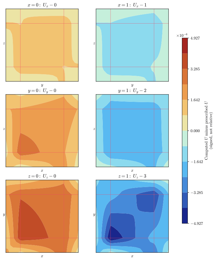
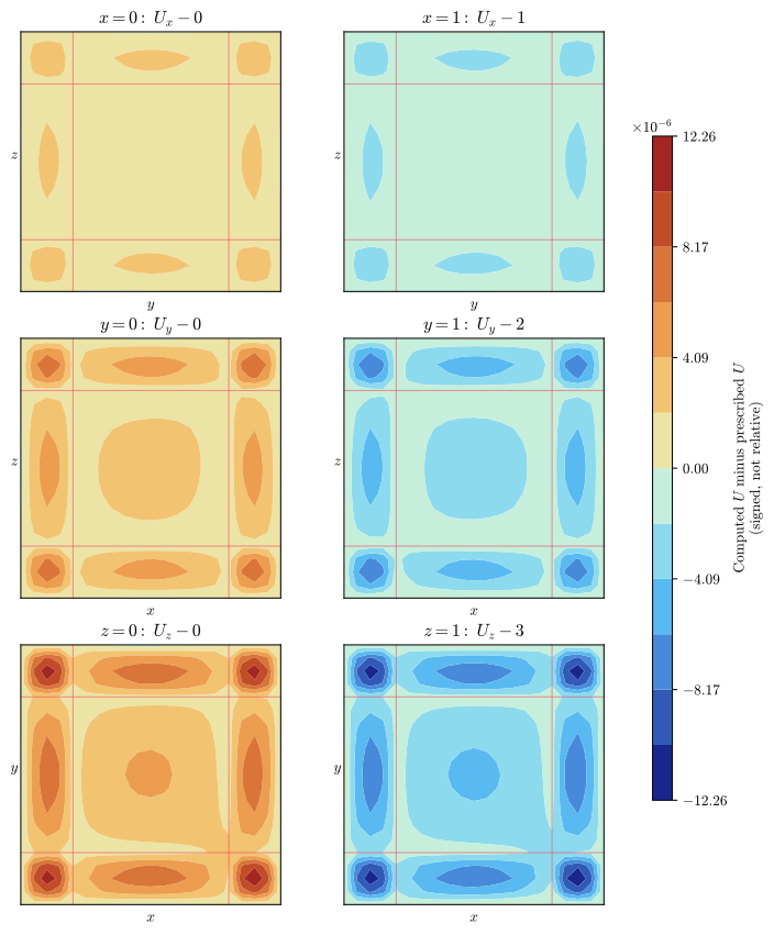
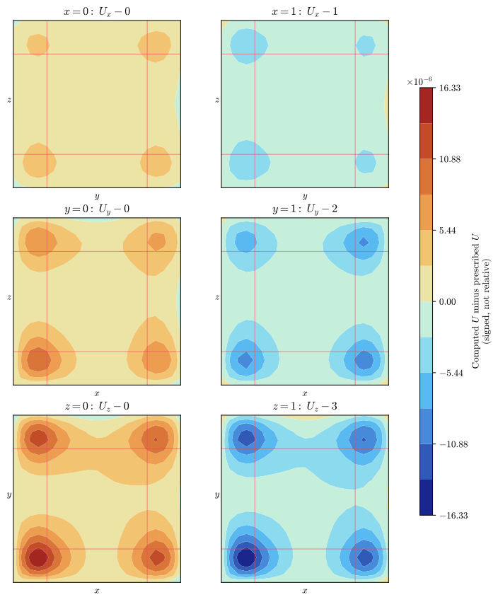
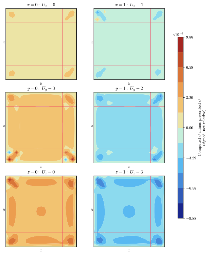
| \(p=2,\ C^1\) | \(0\) | \(16.3 \times 10^{-6}\) | \(13.1 \times 10^{-6}\) | \(38.9 \times 10^{-6}\) |
| \(p=3,\ C^0\) | \(0\) | \(15.1 \times 10^{-6}\) | \(14.2 \times 10^{-6}\) | \(54.6 \times 10^{-6}\) |
| \(p=3,\ C^1\) | \(0\) | \(7.30 \times 10^{-6}\) | \(7.94 \times 10^{-6}\) | \(14.0 \times 10^{-6}\) |
| \(p=3,\ C^2\) | \(0\) | \(9.66 \times 10^{-6}\) | \(3.93 \times 10^{-6}\) | \(28.0 \times 10^{-6}\) |
7.1 Representative results
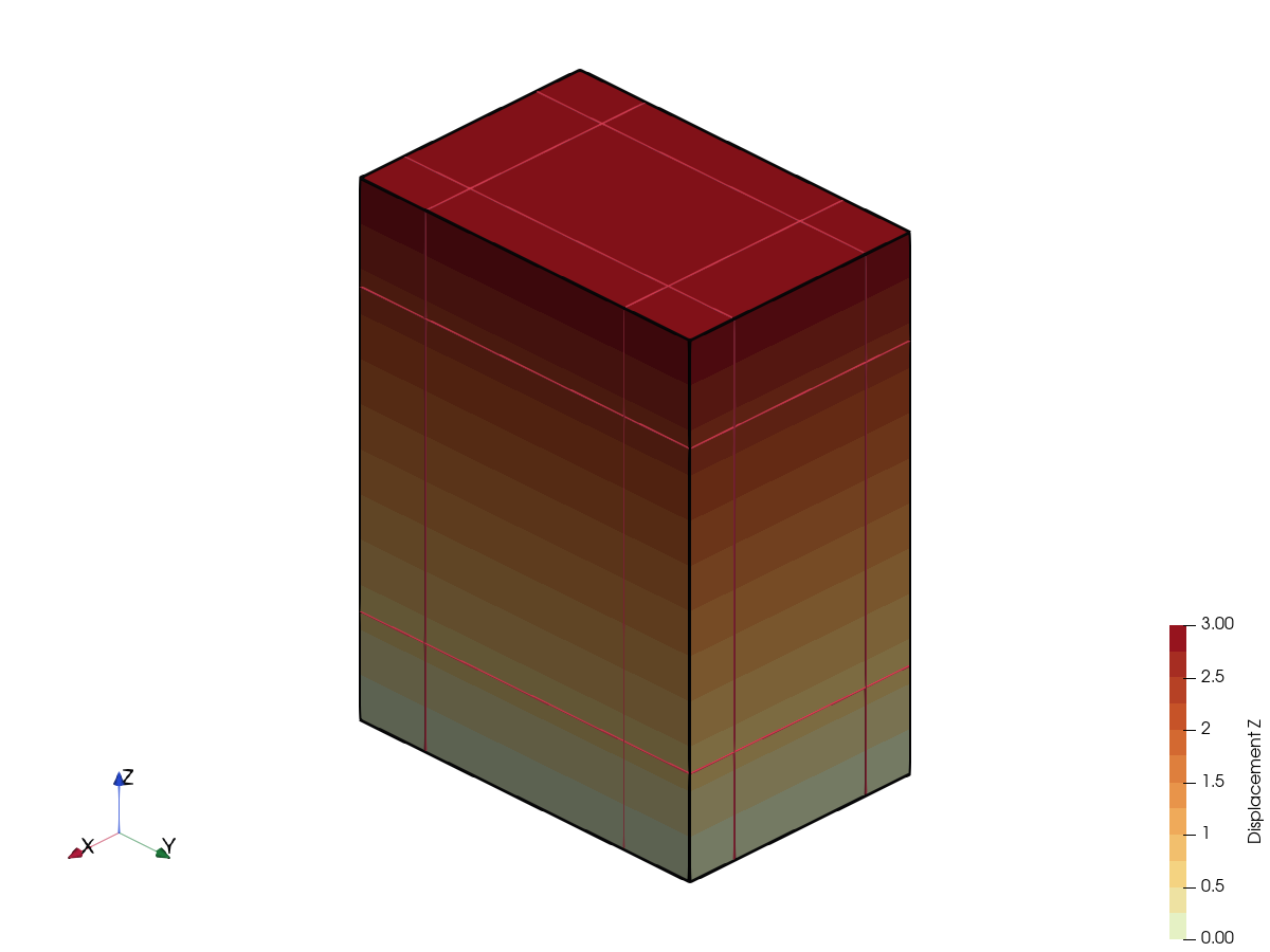
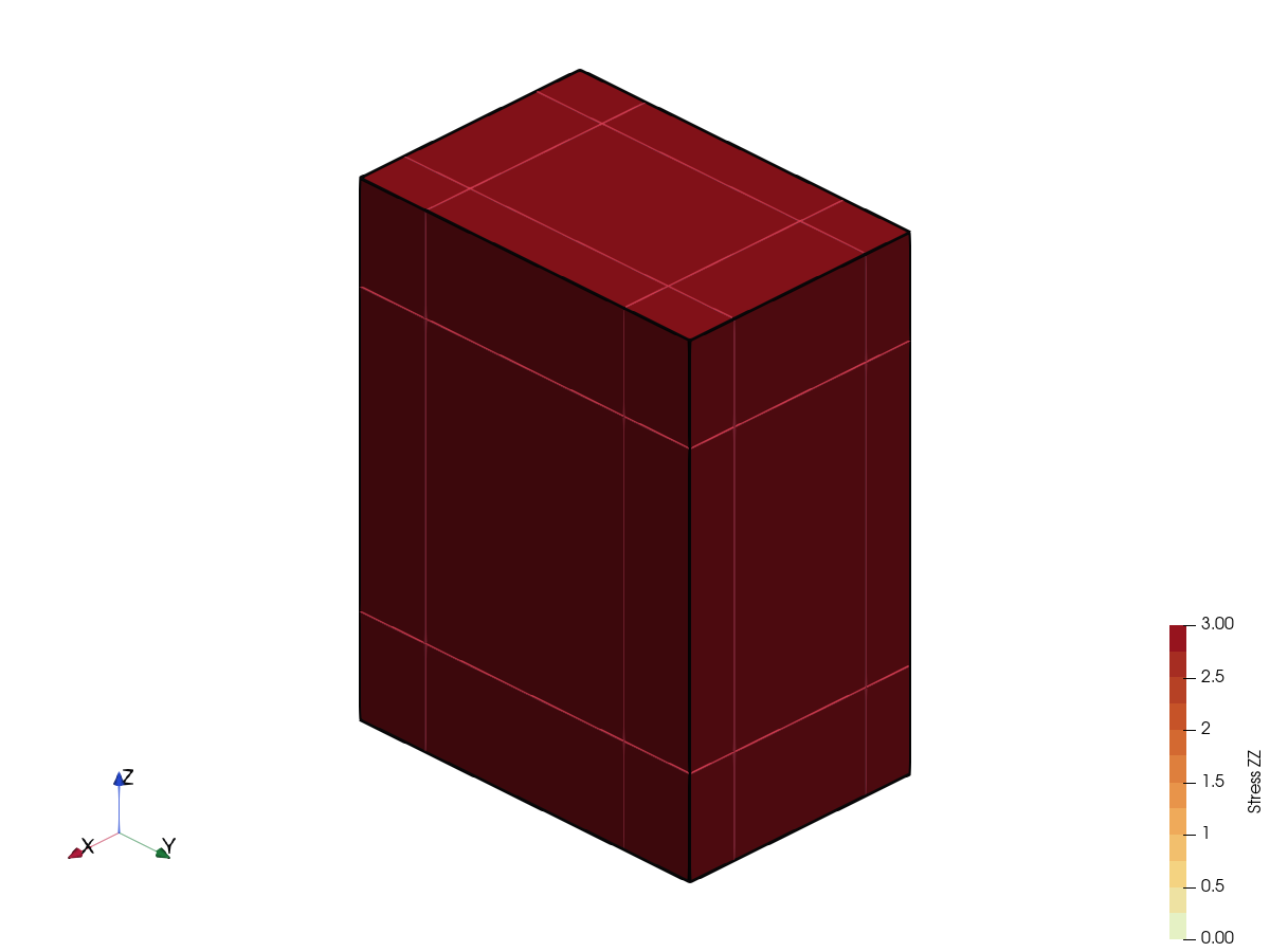
Figure 3 shows the general form of the result produced by every case in the study, using the \(p=2\), \(C^1\) case as a representative example. The geometry is warped by the computed displacement at a scale factor of one. The \(U_z\) field increases from \(0\) at \(z=0\) to \(3\) at \(z=1\), while \(S_{zz}\) remains approximately uniform at \(3\). The orientation triad identifies the view direction, and the warped CAD edges and trimmed Bézier element edges show the discretization on the result surface.
These views establish what the expected affine displacement and constant stress solutions look like, but they are not sufficiently focused to demonstrate verification on their own. The subsequent subsections report the observed boundary-condition and stress residuals for every tested basis.
7.2 Boundary-condition residuals
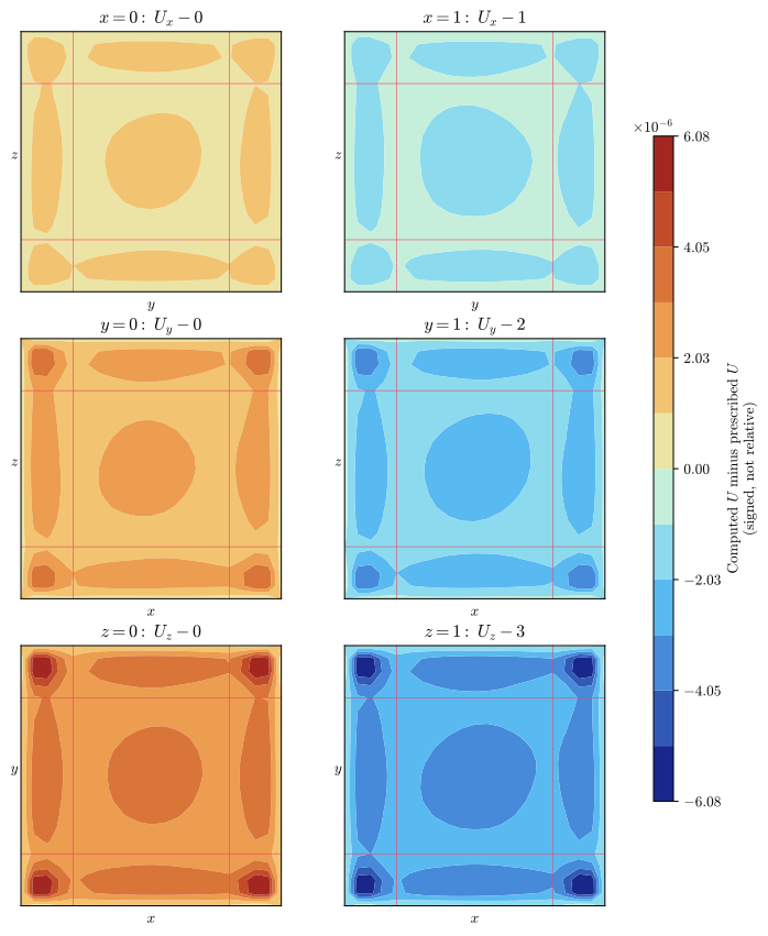
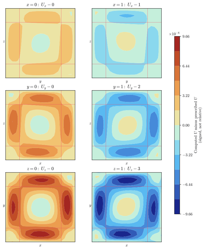
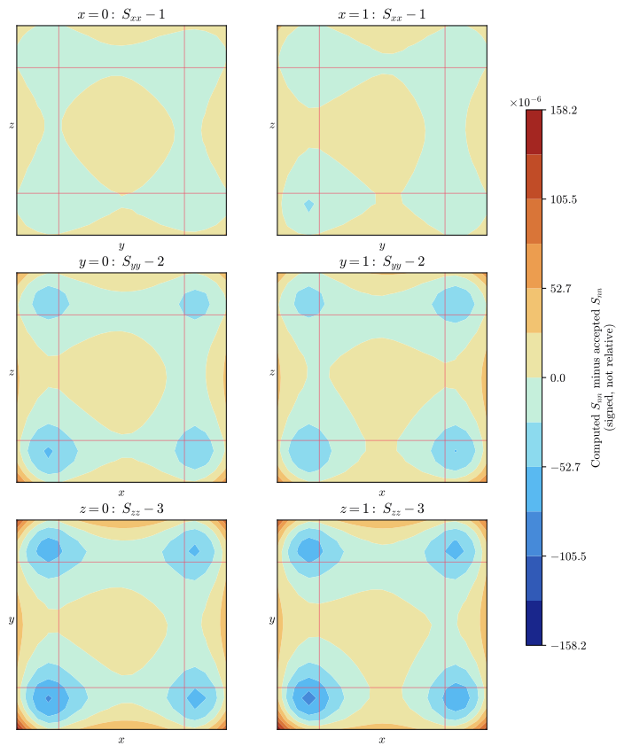
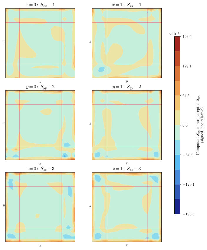
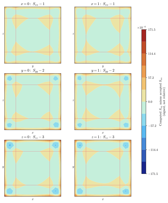
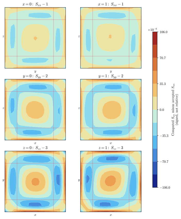
The displacement conditions are imposed weakly on the trimmed boundaries, so the computed displacement at an individual surface point is not expected to equal its prescribed value to machine precision. To expose that behavior, Figure 4 reports the signed error in the prescribed normal component across each face’s \(21\times21\) probe. The residual is the computed displacement minus the prescribed displacement; it is a signed difference in displacement units, not a relative error. Each tab presents one spline basis as an independent figure: rows correspond to the \(x\), \(y\), and \(z\) directions, with the minimum-coordinate face at left and the maximum-coordinate face at right. Each basis uses its own symmetric color limits so its spatial error distribution remains visible. The overlaid lines show where the background mesh planes at \(0.2\) and \(0.8\) intersect each face.
7.3 Boundary normal-stress residuals
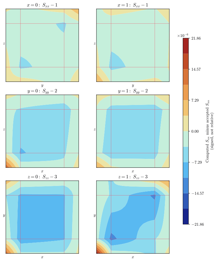
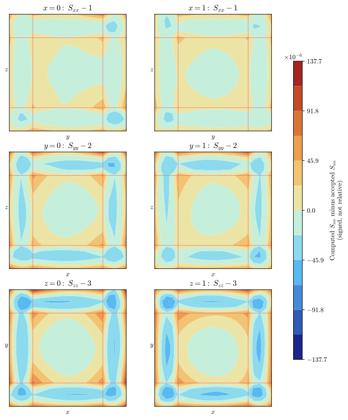
Figure 5 uses the same face probes to show the corresponding normal stress: \(S_{xx}\) on the \(x\) faces, \(S_{yy}\) on the \(y\) faces, and \(S_{zz}\) on the \(z\) faces. The plotted residuals are measured from the accepted values \(1\), \(2\), and \(3\), respectively, so the spatial variation remains visible instead of being obscured by the nearly uniform stress field. They are signed differences in stress units, not relative errors. Each basis again uses its own symmetric color limits. The tab selection is synchronized with the boundary-condition residual figure.
The interior-grid comparison reported in Table 4 remains the full-tensor check: it includes all three normal and all three shear components.
8 Discussion
This study places every displacement condition on a trimmed boundary element while retaining a fully untrimmed element in the cube interior. Agreement on all six faces therefore checks the translation and enforcement of independent zero and nonzero prescribed components without relying on a user subroutine.
The Abaqus output-database comparison is independent of the Coreform IGA probe output: it confirms that every named face element set contains SFM3D3 elements and that the paired nodal displacements reproduce the accepted field. The interior grid then checks that the displacement constraints produce the expected constant normal stress and zero shear stress throughout the volume for each tested degree-continuity combination.
References
[1]
Abaqus materials guide, 2026 FD03. Dassault Systèmes, 2026.
[2]
Abaqus keywords guide, 2026 FD03. Dassault Systèmes, 2026.
[3]
Abaqus analysis guide, 2026 FD03. Dassault Systèmes, 2026.
[4]
Abaqus theory guide, 2026 FD03. Dassault Systèmes, 2026.
Appendix
8.1 Capabilities exercised
The table is generated from current passing artifacts. Each row must satisfy the linked capability card’s evidence contract; declaring a capability in a test does not, by itself, create evidence.
8.2 Download artifacts
Download all verification artifacts (ZIP)
8.2.1 Geometry CAD files
No separate CAD file is required for this problem; the geometry is fully defined in the Abaqus/CAE journal files.
8.2.2 Abaqus/CAE journal files
6 generated Abaqus/CAE journals are available.
Show 6 individual journals
8.3 Supported Abaqus keywords
The deck below is reproduced from the \(p=1\), \(C^0\) test’s Abaqus input file with comments stripped and instance-specific names redacted to <placeholders>.
Noteprescribed_displacement_cube_p1c0.inp - outline
*Heading
*Preprint, echo=NO, model=NO, history=NO, contact=NO
*Include, input=<iga-mesh-inp>
*System
*Material, name=<material>
*Elastic
1.,0.
*User Output Variables
1,
*Step, name=<step>, nlgeom=NO, inc=1, unsymm=YES
*Static, direct
1., 1.,
*Boundary
<node-set>, 1, 1, 1.
*Boundary
<node-set>, 1, 1
*Boundary
<node-set>, 2, 2, 2.
*Boundary
<node-set>, 2, 2
*Boundary
<node-set>, 3, 3, 3.
*Boundary
<node-set>, 3, 3
*Restart, write, frequency=0
*Output, field
*Node Output
U,
*Element Output, position=AVERAGED AT NODES, directions=YES
S,
*Node Output
U
*Output, history, variable=PRESELECT
*End Step
8.4 Provenance
The records below identify the execution environment and verification basis for every CTest artifact reported on this page.
NoteTest_abaqus_verification_prescribed_displacement_cube_p1c0
| Parameter | Value |
|---|---|
| Evidence type | Numerical verification |
| CTest result | Passed (Release) |
| Verification result | Passed — 15/15 enforced criteria passed |
| Test date | 10-Sep-2026 16:03:46 |
| Operating system | Ubuntu 22.04.4 LTS |
| Coreform IGA version | 2026.9+69838 |
| Source revision | d88163e59ac0 |
| Abaqus version | Abaqus 6.26-4 |
NoteTest_abaqus_verification_prescribed_displacement_cube_p2c0
| Parameter | Value |
|---|---|
| Evidence type | Numerical verification |
| CTest result | Passed (Release) |
| Verification result | Passed — 15/15 enforced criteria passed |
| Test date | 10-Sep-2026 16:03:42 |
| Operating system | Ubuntu 22.04.4 LTS |
| Coreform IGA version | 2026.9+69838 |
| Source revision | d88163e59ac0 |
| Abaqus version | Abaqus 6.26-4 |
NoteTest_abaqus_verification_prescribed_displacement_cube_p2c1
| Parameter | Value |
|---|---|
| Evidence type | Numerical verification |
| CTest result | Passed (Release) |
| Verification result | Passed — 15/15 enforced criteria passed |
| Test date | 10-Sep-2026 16:03:43 |
| Operating system | Ubuntu 22.04.4 LTS |
| Coreform IGA version | 2026.9+69838 |
| Source revision | d88163e59ac0 |
| Abaqus version | Abaqus 6.26-4 |
NoteTest_abaqus_verification_prescribed_displacement_cube_p3c0
| Parameter | Value |
|---|---|
| Evidence type | Numerical verification |
| CTest result | Passed (Release) |
| Verification result | Passed — 15/15 enforced criteria passed |
| Test date | 10-Sep-2026 16:03:18 |
| Operating system | Ubuntu 22.04.4 LTS |
| Coreform IGA version | 2026.9+69838 |
| Source revision | d88163e59ac0 |
| Abaqus version | Abaqus 6.26-4 |
NoteTest_abaqus_verification_prescribed_displacement_cube_p3c1
| Parameter | Value |
|---|---|
| Evidence type | Numerical verification |
| CTest result | Passed (Release) |
| Verification result | Passed — 15/15 enforced criteria passed |
| Test date | 10-Sep-2026 16:03:15 |
| Operating system | Ubuntu 22.04.4 LTS |
| Coreform IGA version | 2026.9+69838 |
| Source revision | d88163e59ac0 |
| Abaqus version | Abaqus 6.26-4 |
NoteTest_abaqus_verification_prescribed_displacement_cube_p3c2
| Parameter | Value |
|---|---|
| Evidence type | Numerical verification |
| CTest result | Passed (Release) |
| Verification result | Passed — 15/15 enforced criteria passed |
| Test date | 10-Sep-2026 16:03:38 |
| Operating system | Ubuntu 22.04.4 LTS |
| Coreform IGA version | 2026.9+69838 |
| Source revision | d88163e59ac0 |
| Abaqus version | Abaqus 6.26-4 |