Surface-to-surface contact in a door-lock assembly
A three-part immersed IGA assembly with frictional surface-to-surface contact.
1 Overview
1.1 Purpose
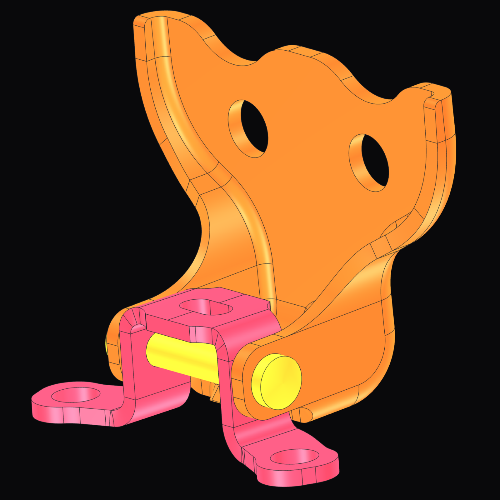
This example demonstrates contact-driven load transfer between three deformable, immersed isogeometric analysis (IGA) parts in an Abaqus/Standard static analysis. The assembly consists of a hinge, a link, and a connecting pin. A prescribed displacement pulls the hinge while the link is held in place, and the load is transferred through the connecting pin.
The problem exercises contact among multiple IGA parts, frictional sliding, large-deformation kinematics, elastic-plastic materials, and reaction-force output.
1.2 Supported contact scope
Coreform IGA for Abaqus currently supports only Abaqus/Standard surface-to-surface contact pairs. Immersed IGA surfaces may be paired with natively meshed Abaqus surfaces. You must explicitly select and pair the main and secondary surfaces for every intended interaction. Self-contact is not yet supported, so the main and secondary surfaces must belong to different bodies.
General contact is also not supported. Do not use General contact (Standard) or rely on an ALL EXTERIOR definition to discover possible contact automatically. Other contact formulations, including node-to-surface contact, are outside the currently supported scope.
The supported surface-to-surface capability remains experimental and may be sensitive to contact-surface selection, surface tessellation, mesh resolution, penalty parameters, and nonlinear solution controls. Convergence of this example does not establish that a different contact model will converge or produce an accurate result. Validate contact behavior, force transfer, and the quantities of interest against a reference solution or a conventional Abaqus discretization before using the results for engineering decisions.
1.3 How Coreform IGA for Abaqus handles contact
To set up a surface-to-surface contact problem, define the contact property, contact surfaces, and surface-to-surface interactions in Abaqus/CAE before creating the Coreform IGA for Abaqus job. During job generation, Coreform IGA for Abaqus retains the explicit contact-pair definitions and identifies the CAD faces referenced by each Abaqus surface. For each selected IGA boundary, the plugin evaluates the trimmed spline boundary and exports a triangulated layer of Abaqus SFM3D3 surface elements. These surface elements provide Abaqus/Standard with conventional element-based surfaces on which its native surface-to-surface contact algorithm can operate.
The nodes of the exported contact surface are additional boundary degrees of freedom rather than control points of the IGA volume. Coreform IGA for Abaqus adds the relevant boundary nodes to the connected IGA user elements and couples their displacement to the spline displacement field with a penalty formulation. Contact forces calculated by Abaqus on the surface elements are therefore transferred through the boundary penalty coupling to the IGA volume. The Abaqus tangential contact penalty and the Coreform IGA for Abaqus boundary coupling penalty serve different purposes: the former enforces the selected friction law, while the latter couples the exported contact surface to the underlying IGA solution.
This construction allows Abaqus’ contact machinery to interact with body-fitted or immersed IGA parts, but it introduces an approximation of the CAD boundary through the exported surface tessellation. Use a contact-surface tessellation and IGA mesh resolution that are fine enough to represent the local curvature and pressure distribution.
1.4 Model definition
The model uses the MMTS consistent unit system recorded in the test artifact and defines two steel materials. Both materials use isotropic elasticity and a two-point, linearly extrapolated plastic hardening definition.
| Property | Weak steel | Strong steel |
|---|---|---|
| Density | \(8.00 \times 10^{-9}\ \mathrm{tonne}/\mathrm{mm}^3\) | \(8.00 \times 10^{-9}\ \mathrm{tonne}/\mathrm{mm}^3\) |
| Young’s modulus | \(200 \times 10^{3}\ MPa\) | \(200 \times 10^{3}\ MPa\) |
| Poisson’s ratio | \(0.29\) | \(0.29\) |
| Initial yield point | \(1.50 \times 10^{3}\ MPa\) at plastic strain \(0\) | \(2.00 \times 10^{3}\ MPa\) at plastic strain \(0\) |
| Second hardening point | \(150 \times 10^{3}\ MPa\) at plastic strain \(10\) | \(200 \times 10^{3}\ MPa\) at plastic strain \(10\) |
The pin is partitioned into the cylindrical section and the two end caps. The cylindrical section uses the strong steel material and the two end caps use the weak steel material. The hinge and link use weak steel throughout.
| Analysis setting | Value |
|---|---|
| Unit system | mm, N, MPa |
| Model | Door-Lock |
| Procedure | Static, General |
| Geometric nonlinearity | On |
| Initial increment | \(0.1\) |
| Minimum increment | \(10.0 \times 10^{-9}\) |
| Link boundary condition | Pinned |
| Hinge displacement \((U_1, U_2, U_3)\) | (0, 0, 5) mm |
1.5 Contact definition
The model uses an isotropic penalty-friction interaction property. The normal contact behavior uses the Abaqus defaults.
| Contact setting | Value |
|---|---|
| Formulation | surface-surface |
| Interaction type | friction |
| Friction coefficient | \(0.3\) |
| Maximum elastic-slip fraction | \(5.00 \times 10^{-3}\) |
| Sliding | Finite |
| Include surface thickness | Yes |
| Interaction | Main surface |
| — | — |
| pin_to_hinge_contact | Pin |
| pin_to_link_contact | Pin |
| hinge_to_link_contact | Hinge |
All three interactions are active from the Initial step. They apply no initial overclosure adjustment and omit a user-specified initial clearance.
1.6 IGA discretization
| Discretization setting | Value |
|---|---|
| Mesh | Immersed rectilinear |
| Spline degree | \(2\) |
| Continuity | \(C^1\) |
| Element size \((x, y, z)\) | (2, 2, 2) mm |
| Padding elements \((x, y, z)\) | (2, 2, 2) |
Boundary tessellation is resolved by the mesher from the geometry and element size; it is no longer a user-specified discretization setting.
1.7 Output and test result
The field-output request and reaction-force history request are defined by the test:
| Output | Value |
|---|---|
| Field variables | S, U, PEEQ |
| Field position | Averaged at nodes |
| History component | RF3 |
| History region | hold_link_surfaces |
| Summed history regions | \(666\) |
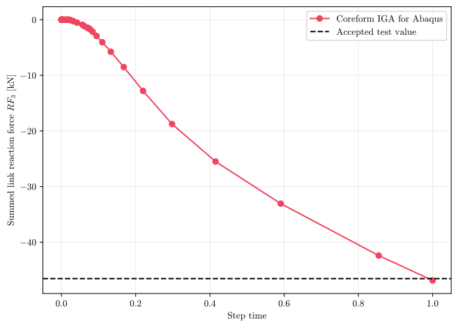
At the end of the prescribed displacement, the summed link reaction force is \(-46.883\ kN\).