Nearly incompressible elasticity — Cook’s membrane
A large-deformation Cook’s membrane example using the alpha locking-free formulation.
1 Overview
Nearly incompressible materials can cause volumetric locking in a displacement-only formulation, making the computed structure artificially stiff. Coreform’s locking-free formulation introduces an independent pressure field for the volumetric response, while displacement represents the distortional response. The volume constraint is enforced in a weak, averaged sense rather than point by point.
This example applies the formulation to a quadratic, body-fitted Cook’s membrane model undergoing large deformation. It uses a nearly incompressible material and Coreform’s compressible Neo-Hookean material model.
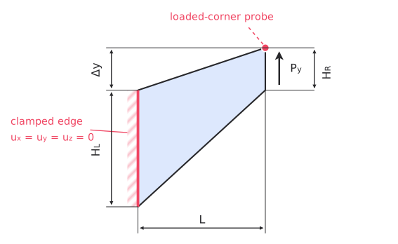
Figure 1 shows a plan view of the trapezoidal geometry and applied boundary conditions. The left face is clamped, out-of-plane displacement is fixed throughout the body, and an upward resultant shear load is applied to the right face. The upper loaded corner is the displacement-probe location; the out-of-plane thickness \(t\) listed below is not shown. All dimensional values use the MMTS consistent unit system.
| Property | Value |
|---|---|
| Horizontal span, \(L\) | \(48\ mm\) |
| Left height, \(H_L\) | \(44\ mm\) |
| Right height, \(H_R\) | \(16\ mm\) |
| Upper-edge vertical offset, \(\Delta y\) | \(16\ mm\) |
| Extruded thickness, \(t\) | \(1.91516\ mm\) |
| Young’s modulus, \(E\) | \(240.565\ MPa\) |
| Poisson’s ratio, \(\nu\) | \(0.49999\) |
| Applied resultant shear load, \(P_y\) | \(6.25\ N\) |
| Geometric nonlinearity | On |
1.1 Performance and limitations
The locking-free formulation requires additional local pressure projection, residual, and tangent assembly. The default statically condenses the pressure coefficients before global assembly, so it does not add global pressure degrees of freedom. Immersed pressure-cell aggregation can enlarge the displacement coupling associated with one user element, increasing solution time and memory use.
This example demonstrates unreleased alpha functionality, not a generally supported production workflow.
2 Formulation
The default displacement–pressure pair is \(U(p,C^{p-2},h)/P(0,C^{-1},h)\): the displacement continuity is reduced by one from maximum continuity and each fine pressure cell has one discontinuous constant coefficient. The pressure field supplies the hydrostatic stress and relieves the displacement field from the constraint that causes volumetric locking. Pressure coefficients are eliminated locally by static condensation. No GLS, SUPG, VMS, or pressure-gradient stabilization term is enabled by default.
For an immersed domain, a pressure cell with insufficient physical support is aggregated with a nearby admissible donor before condensation. This cut-cell treatment prevents a nearly singular local pressure projection; it is separate from residual-based pressure stabilization.
2.1 Material behavior
The material implementation depends on the Abaqus geometric-nonlinearity setting:
| Abaqus setting | Material behavior |
|---|---|
NLGEOM=OFF |
Uses Coreform’s in-house isotropic linear-elastic model through UEL. |
NLGEOM=ON |
Uses Coreform’s in-house compressible Neo-Hookean model through UEL. |
All locking-free formulations use UEL. The UEL selects the material implementation from the kinematics of each element call: NLGEOM=OFF uses linear elasticity, and NLGEOM=ON uses Neo-Hookean elasticity. A job may therefore begin with a small-deformation step and enable finite deformation in a later step. Abaqus carries an enabled NLGEOM setting into subsequent steps, so those steps may omit the attribute. Plasticity is not yet supported for locking-free UEL elements.
3 Activate the locking-free formulation
Set USE_LOCKING_FREE=1 before starting Coreform IGA for Abaqus, then create or regenerate the Coreform IGA job. The environment variable is read during export; setting it only when submitting an existing input deck is too late.
On Linux:
export USE_LOCKING_FREE=1
/opt/Coreform-IGA-2026.7/bin/coreform_iga
On Windows Command Prompt:
set USE_LOCKING_FREE=1
"C:\Program Files\Coreform IGA 2026.7\coreform_iga.bat"
Set USE_LOCKING_FREE=0, or remove the environment variable, to return to the regular formulation.
4 Download and run the example
Download the Abaqus/CAE journal file below to reconstruct the model and generate the input artifacts used by this example.
Run the journal from a new, writable directory so its output files are easy to identify. Set USE_LOCKING_FREE=1 before starting Abaqus/CAE, as described above, and use Abaqus/CAE’s recover option rather than File > Run Script. Abaqus recommends recover for .jnl files; running a journal as an ordinary script can produce an incomplete model database.
On Linux, the Coreform launcher changes to RUNTIME_DIR before starting Abaqus/CAE, so set it to the directory containing the downloaded journal:
mkdir -p cooks-membrane
cd cooks-membrane
# Save cooks_membrane.jnl in this directory before continuing.
export USE_LOCKING_FREE=1
export RUNTIME_DIR="$PWD"
/opt/Coreform-IGA-2026.7/bin/coreform_iga recover="$PWD/cooks_membrane.jnl"
On Windows Command Prompt:
mkdir cooks-membrane
cd /d cooks-membrane
rem Save cooks_membrane.jnl in this directory before continuing.
set USE_LOCKING_FREE=1
"C:\Program Files\Coreform IGA 2026.7\coreform_iga.bat" recover="%CD%\cooks_membrane.jnl"
Abaqus/CAE executes the journal during startup. Wait for model recovery and the Coreform exports to finish before closing Abaqus/CAE. The journal produces the following files in the working directory:
| File | Contents |
|---|---|
cooks_membrane.cae |
Reconstructed Abaqus/CAE model database, including the Coreform IGA mesh and job definitions. |
cooks_membrane.cf |
Coreform model export consumed by Coreform IGA Mesh. |
cooks_membrane.inp |
Abaqus simulation input exported from the CAE model for the subsequent interop step. |
cooks_membrane.jnl |
Abaqus/CAE recovery journal associated with the saved model database. |
abaqus.rpy |
Abaqus/CAE session replay log. Abaqus may add a numeric suffix if a replay log already exists. |
These are model-generation artifacts, not analysis results.
4.1 Run Abaqus/Standard
Keep the recovered model open in the same Abaqus/CAE session and complete the analysis as follows:
Switch to the Job module.
Click the Coreform IGA Job Manager icon to open the Coreform IGA for Abaqus - Job Manager.
Select the
cooks_membranejob and click Submit. Use the Coreform job manager, not the standard Abaqus job manager. The Coreform Submit action rebuilds the IGA mesh, runs the Abaqus interop translation, and then submits the translatedcooks_membrane.inpdeck to Abaqus/Standard. It is not necessary to click Build Mesh first.Leave Abaqus/CAE running until the job status changes to Completed. A successful run prints messages similar to the following in the Abaqus/CAE message area:
Job cooks_membrane: Analysis Input File Processor completed successfully.
Job cooks_membrane: Abaqus/Standard completed successfully.
Job cooks_membrane completed successfully.
With
cooks_membranestill selected in the Coreform job manager, click Results to opencooks_membrane_iga.odbin the Visualization module. The standard Abaqus output database,cooks_membrane.odb, can also be opened with File > Open.
The completed workflow produces these primary result artifacts:
| File | Contents |
|---|---|
cooks_membrane.odb |
Standard Abaqus output database. |
cooks_membrane_iga.odb |
IGA results mapped to the visualization mesh. |
probe_data.json |
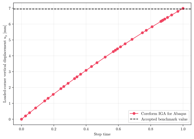
Probe histories, including the loaded-corner displacement plotted below. |
The working directory also contains the Coreform mesh database and translated input-deck files, as well as the usual Abaqus/Standard status and diagnostic files such as .dat, .msg, and .sta.
5 Expected result
The vertical displacement at the loaded upper corner is \(u_y = 6.98868\) \(\mathrm{mm}\).