3 Structural Modal Analysis
3.1 Frequency Extraction
3.1.1 Frequency Extraction of Free Circular Plate
3.1.1.1 Objective
This verification problem shows that the Flex method is able to calculate several of the lowest fundamental frequencies of an unconstrained circular plate.
This problem is chosen as a verification problem because while exact solutions known they are quite challenging to derive and thus this problem represents, perhaps, the simplest structural modal problem for which known solutions exist yet it is still preferred, in practice, to produce a numerical approximation.
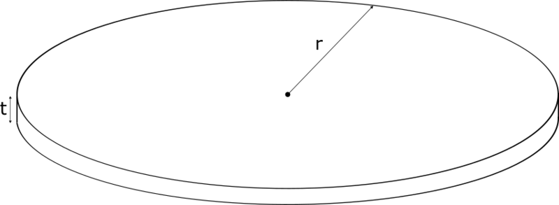
3.1.1.2 Geometry Description
The geometry for this problem is a circular plate shown in figure 43. The parameters used to describe this geometry are provided in table 45.
Parameter
Value
t
0.01
r
1
3.1.1.3 External Interactions
There are no boundary conditions applied to the circular plate (i.e., “free vibration”).
3.1.1.4 Material Description
Dimension
Value
Young's Modulus
Poisson's Ratio
0.3
Density
1
3.1.1.5 Method
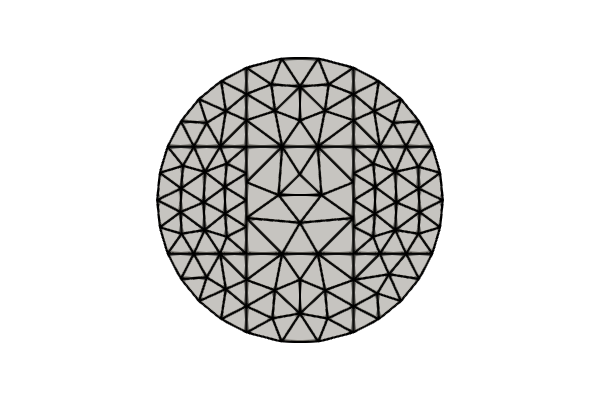
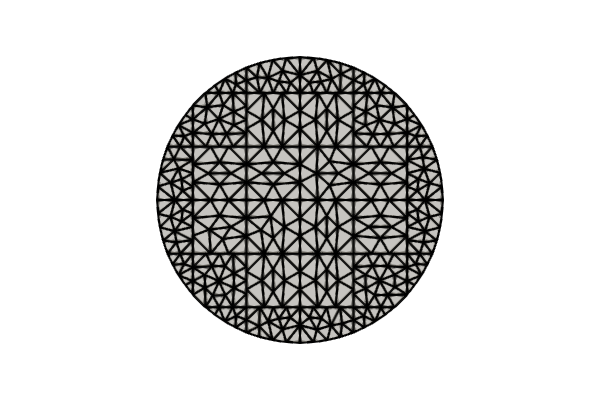
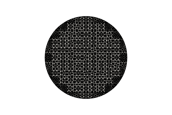
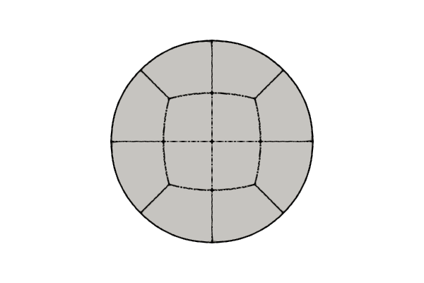
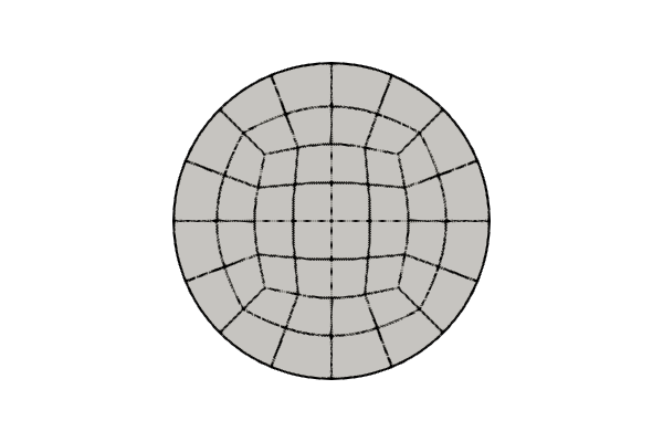
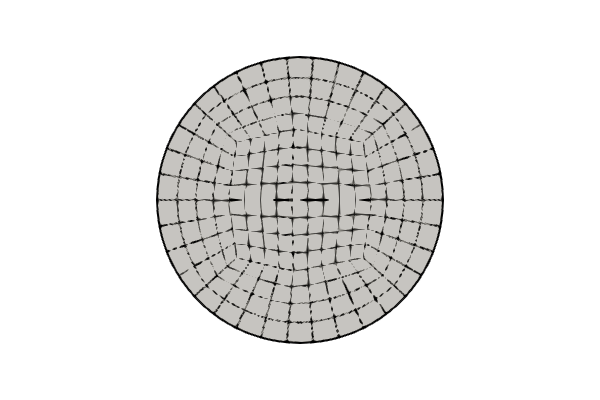
Results for this problem were computed using two approaches, each using Coreform IGA. One approach consisted of a traditional bodyfit-meshing approach while the other utilizes an immersed meshing approach. In addition, three levels of refinement were performed using each approach. These refinement levels are listed in table 47. A quadratic basis with maximal continuity was used in each case.
Refinement
Quadrature points
DOF
Immersed
Bodyfit
Immersed
Bodyfit
Coarse
243
324
225
360
Medium
864
1296
540
864
Fine
2937
5616
1413
2700
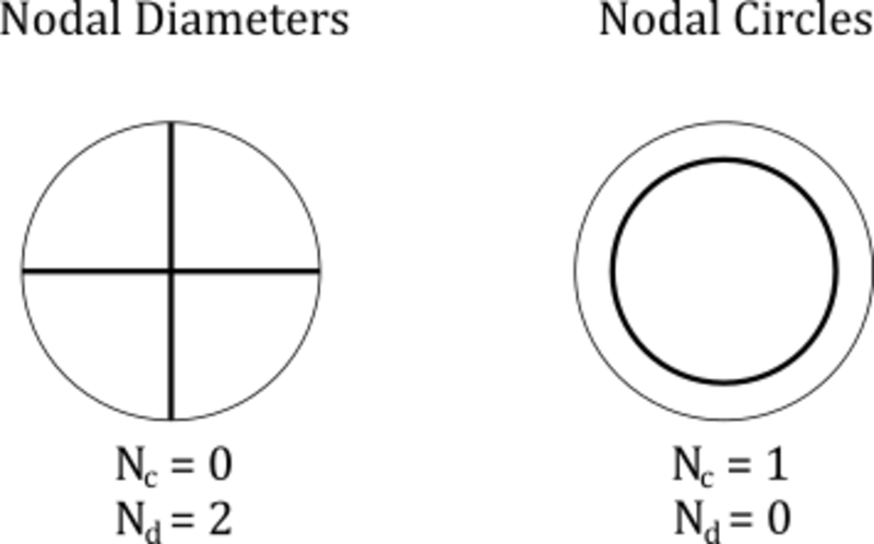
Results from both bodyfit and immersed meshes were compared against the analytic solution to the first fundamental frequency of a free vibrating circular plate. For a circular plate with radius , thickness , density , Young’s modulus , and Poisson’s ratio , the analytic solution for the natural frequencies in a vacuum are where is the non-dimensional frequency parameter and is the flexural rigidity. For a circular plate, the flexural rigidity is The non-dimensional frequency parameter is tabulated in the literature for values of and , where is the number of nodal circles and is the number of nodal diameters (see figure 45). A shortened list of calculated non-dimensional frequency parameters is shown in table 48.
Figure 45: Examples of nodal circles () and nodal circles (). The bolded lines represent the nodal lines of the associated eigenmode.
0
1
2
3.00052
0
2
5
6.20025
0
3
8
9.36751
0
4
11
12.5227
0
5
14
15.6727
1
1
3
4.52488
1
2
6
7.7338
1
3
9
10.9068
1
4
12
14.0667
1
5
15
17.2203
2
0
1
2.31481
2
1
4
5.93802
2
2
7
9.18511
2
3
10
12.3817
2
4
13
15.5575
2
5
16
18.722
3.1.1.6 Results
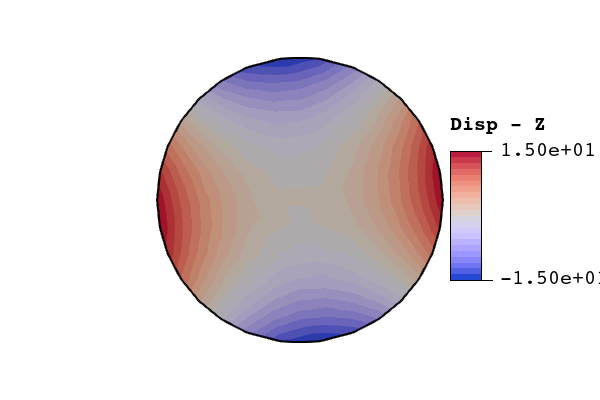
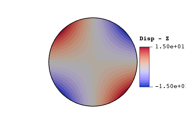
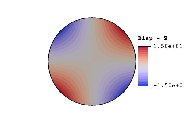

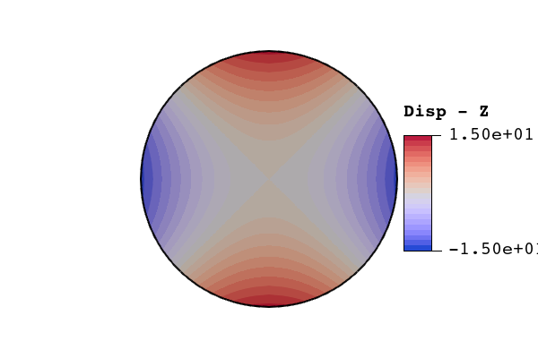
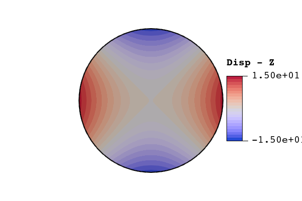
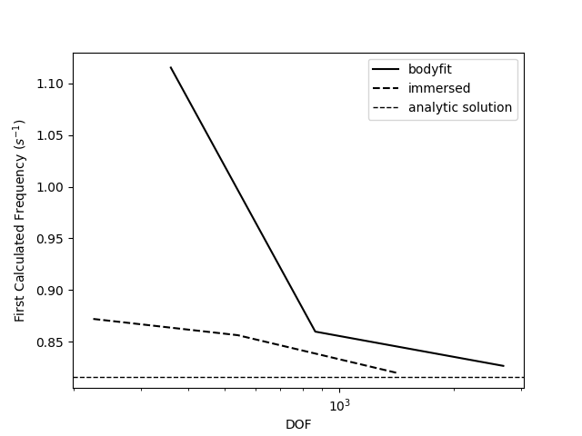
Table 49 shows the calculated first frequency of the finest mesh for both approaches, as well as the relative error between each solution and the analytic solution.
Approach
Calculated Frequency ()
Relative Error (%)
Immersed
0.8220
0.72 %
Bodyfit
0.8266
1.29 %
Table 49: Relative error in fine mesh solutions for both approaches
Table 50 shows the solution characteristics of the finest mesh for both approaches.
Approach
Initialization Time (s)
Linear Equation Time (s)
Nonlinear Equation Time (s)
Solver Time (s)
immersed
1.22e-05
0.35
0.36
1.48
bodyfit
1.72e-05
0.39
1.31
2.50
Table 50: Solution characteristics for fine mesh solutions for both approaches