2 Solid Mechanics
2.1 Linear Stress Analysis
2.1.5 Stresses in long pressurized pipe with butt-welded supporting trunnion pipes |
2.1.6 Stress Concentrations: filleted square shoulder of rectangular section |
2.1.1 Cantilever beam with end shear load
2.1.1.1 Objective
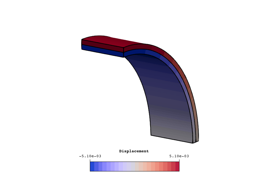
This verification problem demonstrates that higher-order elements can capture the exact solution of a simple cantilever beam problem with coarse meshes. In this problem we analyse the normal and shear stress profiles of a cantilever beam with a square cross-section that is subjected to a tip load using quadratic and cubic basis functions. The results show that both choices of basis functions exactly capture the axial stress and that cubic elements capture both the axial and shear stresses exactly on any mesh.
Although real world engineering problems will not in general have solutions that can be captured exactly with quadratic or cubic basis functions, these higher-order functions will typically be more accurate for a given number of degrees of freedom. This allows coarser meshes to be used in simulations, which can lead to reduced computational cost in many problems.
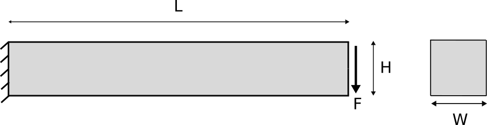
2.1.1.2 Geometry Description
2.1.1.3 External Interactions
A transverse shear traction is applied at the free end of the beam with an average shear stress of in the direction. As the cross-sectional area is , the total applied force is . The shear traction applied to the tip is distributed according to the parabolic solution from Euler–Bernoulli beam theory given in equation , to facilitate precise quantitative accuracy testing. The cantilever support at the fixed end is modeled by fixing displacement in both transverse directions ( and ), and applying a linearly-varying pressure distribution, coming from the Euler–Bernoulli axial stress solution given in equation . The remaining rigid modes are eliminated by constraining axial displacement at only the corners of the cantilever support cross-section. Although the Euler–Bernoulli solution is formally derived through an assumption of cross-sections remaining planar (alongside other approximations), that does not hold exactly for the full three-dimensional displacement solution, and the support cross-section needs to remain free to warp in the axial direction. The remaining rigid modes are eliminated by constraining axial displacement at only the corners of the cantilever support cross-section.
Due to St. Venant’s principle, qualitatively-similar results could be obtained using a fixed boundary condition for the cantilever support and a uniformly-distributed shear traction for the tip load. However, the cubic solution would no longer be exact and significant deviations from the beam-theory solution would occur near the ends of the beam.
2.1.1.4 Material Description
2.1.1.5 Method
2.1.1.6 Solution Characteristics
Since the cross-section of the beam is a square and is composed of a single homogenous material the neutral axis is located at the center of the beam. Thus the normal stress profile can be computed as where is the moment at the axial location being probed and is the area moment of inertia of the cross-section, which is given by for a rectangle. The shear stress profile can be calculated as In the present problem, the shear stress calculation can be simplified to which we note is a parabolic distribution with bounds
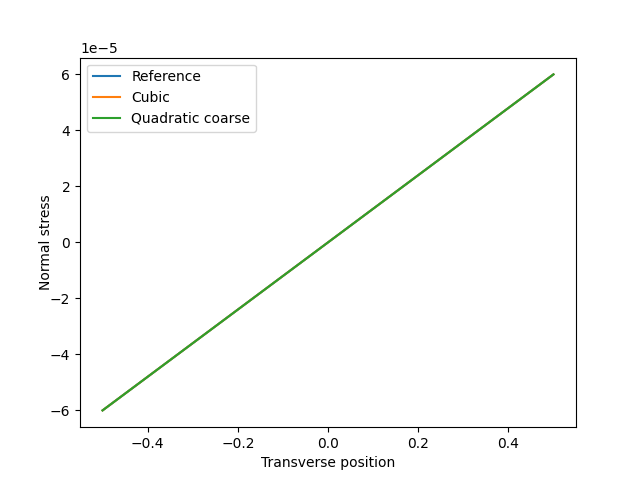
2.1.1.7 Results
2.1.2 Composite cantilever beam with end shear load
2.1.2.1 Objective
This verification problem demonstrates the accuracy of tied constraints between adjacent parts by computing the stress profile through a composite cantiliver beam composed of a stiff and flexible section. The normal and shear stress are compared to an exact reference solution.
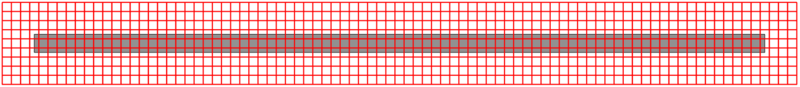
Tied constraints play a critical role when computing results for assemblies using the flex method. In the typical body-fitted approach for assemblies, adjacent parts are often tied together by creating a conformal mesh between the two parts and specifying that coincident nodes at the interface map to the same degrees of freedom. For the flex approach, adjacent parts will each have a different background spline, which in general will not align or share coincident points at the interface. Because of this, tied constraints are used to tie adjacent parts together. In this simple problem, two adjacent cantilever beams are tied together and then subjected to an end load. Results are computed for two cases. In the first case, the background mesh for each section has the same element size. For the second case, the element sizes are different. The results for both cases show that these interfaces can be accurately modeled with the flex method’s tied constraint approach.
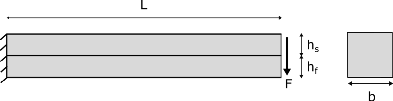
2.1.2.2 Geometry Description
Figure 5: A sketch of the composite cantilever beam showing the stiff and flexible sections that comprise the beam.
Dimension
Value
2.1.2.3 External Interactions
Displacements in the transverse ( and ) directions are contrained on the fixed end of the cantilever beam. The axial displacement is only constrained at the corners of the cantilever support face of the beam’s lower section, to remove rigid modes, while the analytical distribution of axial stress from Euler–Bernoulli beam theory given in equation is applied on the fixed end instead of constraining axial displacement. This is because the analytical solution depends on allowing cross-sections to warp slightly, and we want to be able to perform precise testing of the method’s accuracy. A transverse shear traction is applied at the free end of the beam with a non-dimensional average shear stress of , as shown in figure 5. The beam has a cross-sectional area of , which results in a total applied force of . The traction is distributed according to the analtyical beam-theory solution given in equation , to facilitate accuracy testing. The interface between the two sections is modeled as a material interface, using a dimensionless penalty scale factor of . This is selected higher than the default value recommended for practical analyses, to enable precise comparisons with the analytical solution.
2.1.2.4 Material Description
Property
Flexible
Stiff
Young's Modulus
Poisson's Ratio
Table 4: The non-dimensional material properties for the stiff and flexible layers of the cantilever beam.
2.1.2.5 Method
2.1.2.6 Solution Characteristics
A reference solution for the composite beam can be calculated using the transformed section method, wherein the geometry of the beam is transformed into an imaginary section of uniform material with equivalent elastic properties. We assume here that the notional uniform beam material is equivalent to the material found in the composite beam’s flexible section, so we transform only the geometry of the stiffer material.
The normal stress profile can then be calculated as
where is the distance to the neutral axis of the section and is radius of curvature. Intermediate calculations can be computed via the following expressions:
The shear stress profile can then be calculated as
where intermediate calculations can be computed via the following expressions:
2.1.2.7 Results
The normal stress is plotted along a transverse line at a point midway along the length of the beam in figure 7. The reference solution given in equation is also plotted. All plots are coincident because both quadratic and cubic basis functions are able to represent the solution exactly.
Figure 7: Normal stress profiles. The computed normal stress is coincident with the reference solution in all cases.

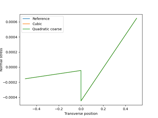
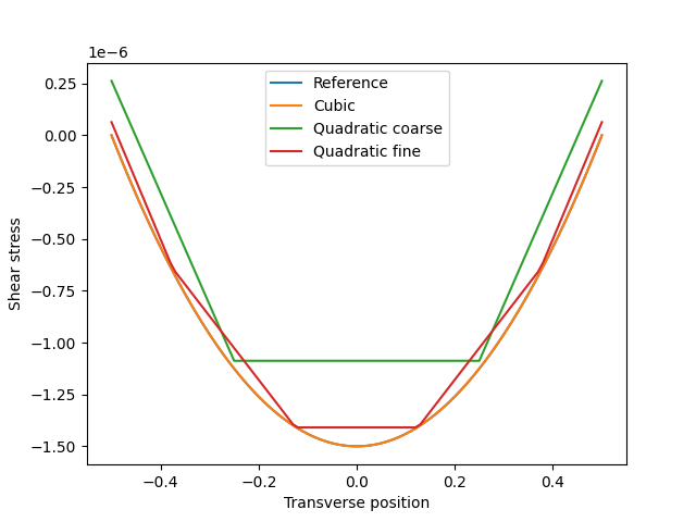
Figure 8: Shear stress profiles. The shear stress computed with the cubic basis is coincident with the reference solution in all cases.
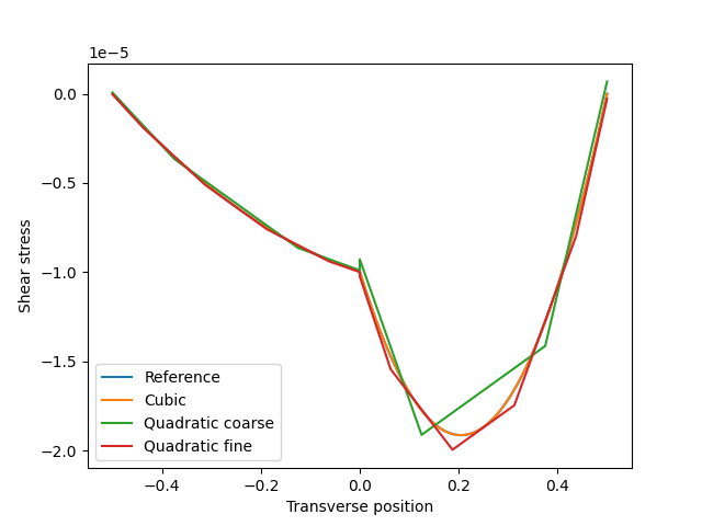
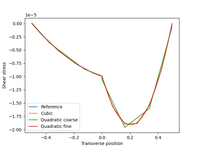
In all cases, the interface between the stiff and flexible sections of the beam was modeled as a tied constraint. These results demonstrate that we are able to accurately represent material interfaces with tied constraints.
2.1.3 Infinite plate with a hole
2.1.3.1 Objective
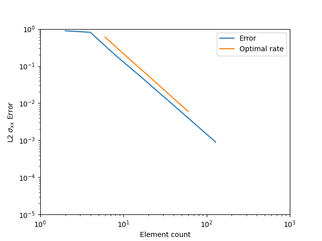
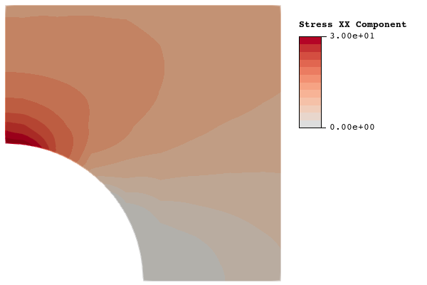
This verification problem shows that the Flex method is able to achieve optimal theoretical mesh convergence rates on the well-known infinite plate with a hole benchmark problem.
This problem is chosen as a verification problem not only because the exact solution is known, but in particular because the geometry includes a hole. The presence of a hole in the geometry presents two problem features that are critical for verification of flex-method stress analysis. First, the hole will produce a stress concentration. Second, the hole will require elements of the background spline to be trimmed in the area of the stress concentration. Accurate representation of stresses near features that produce stress concentrations is critical for stress analysis, and such features will almost always produce trimmed elements. The results presented for this problem show that we are able to achieve theoretical mesh convergence with trimmed elements. We also show that stress gradients can be captured to a reasonable level of accuracy on relatively coarse meshes. These results show that the flex method is a poweful tool for stress analyis of complex parts.
2.1.3.2 Geometry Description
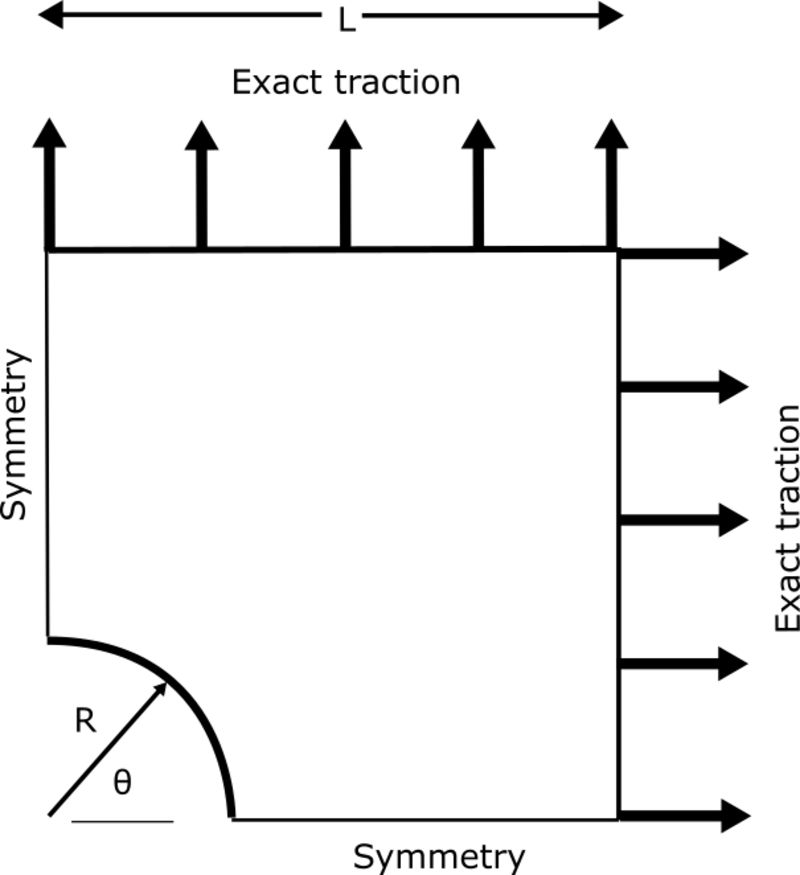
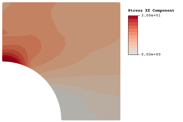
The in-plane geometry for this problem is a quarter-symmetry representation of a square plate with a hole in the center, shown in figure 9. For this problem, and . The out-of-plane thickness is selected to be the mesh element size in each computation, so that there is always only one element in the thickness direction.
Figure 9: A quarter-symmetry representation of a infinite plate with a hole.
2.1.3.3 External Interactions
The model is constrained using symmetry boundary conditions on the left and bottom surfaces, and plane strain deformations are enforced by constraining out-of-plane displacements on both the front and back surfaces. The exact stress is given by in a polar coordinate system with the origin at the center of the hole, where is the traction applied in the direction at infinity. This stress is used to apply the exact tractions on the top and right surfaces, as shown in figure 9.
2.1.3.4 Material Description
2.1.3.5 Method
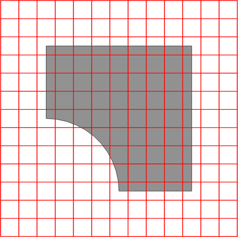
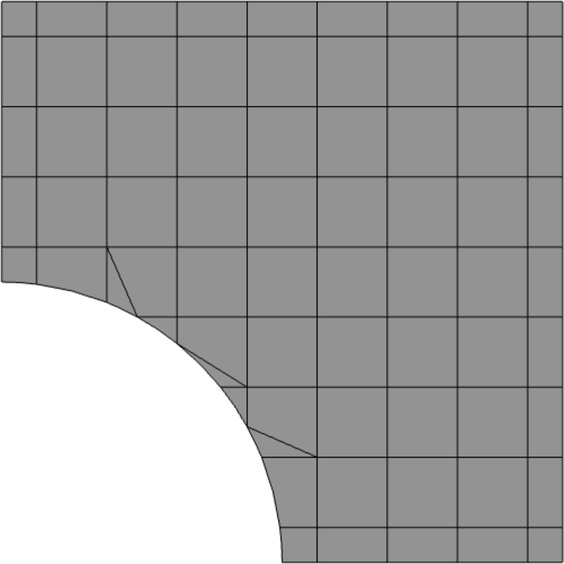
Figure 10: The background mesh for mesh #3. There are approximately eight elements along the long edges of the part.

2.1.3.6 Results

2.1.4 Torsion of a hollow cylinder
2.1.4.1 Objective
This verification problem demonstrates that higher-order elements, and the flex representation method, can accurately compute torsion problems on curved domains even with coarse meshes. Although real world engineering problems will not in general have solutions that can be captured exactly with quadratic or cubic basis functions, these higher-order functions will typically be more accurate for a given number of degrees of freedom. This allows coarser meshes to be used in simulations, which can lead to reduced computational cost in many problems.
2.1.4.2 Geometry Description
2.1.4.3 External Interactions
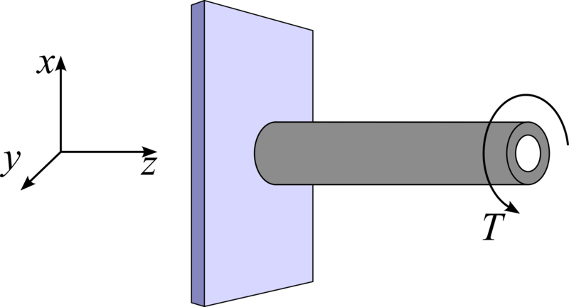
Figure 14: Schematic of the problem definition, the shaft is held fixed at and a torque is applied at .
2.1.4.4 Material Description
2.1.4.5 Method
Label
Refinement Level
0
1
6
10
0.100
1.00
1.00
1
2
12
20
0.050
0.50
0.50
2
4
24
40
0.025
0.25
0.25
Table 10: Number of elements in the bodyfit meshing strategy. The approximate element sizes are provided in the final three columns, denoted as .
Label
Refinement Level
0
0.100
0.100
1.00
1
0.050
0.050
0.50
2
0.025
0.025
0.25
Table 10: Element sizes for the immersed rectilinear meshing strategy.
2.1.4.6 Solution Characteristics
Beam torsion is a classical set of problems, typically introduced in undergraduate mechanical engineering courses. What follows is a standard discussion of beam torsion analysis, as paraphrased from [1].
The shearing strain, , at some radial distance from the centerline of a cantilevered cylindrical shaft of length , that has been rotated about its centerline by radians is
It follows that the maximum shear stress will occur when at the outer surface of the shaft’s cross-section,
allowing us to rewrite equation as
Assuming that the applied torque, , results in a stress state where no yielding has occured (i.e., remains in the elastic regime) and the rotations are small, we can apply Hooke’s law for shear stress and strains
where is the shear modulus of the material. Multiplying both sides of equation by and using the relationship of equation we obtain
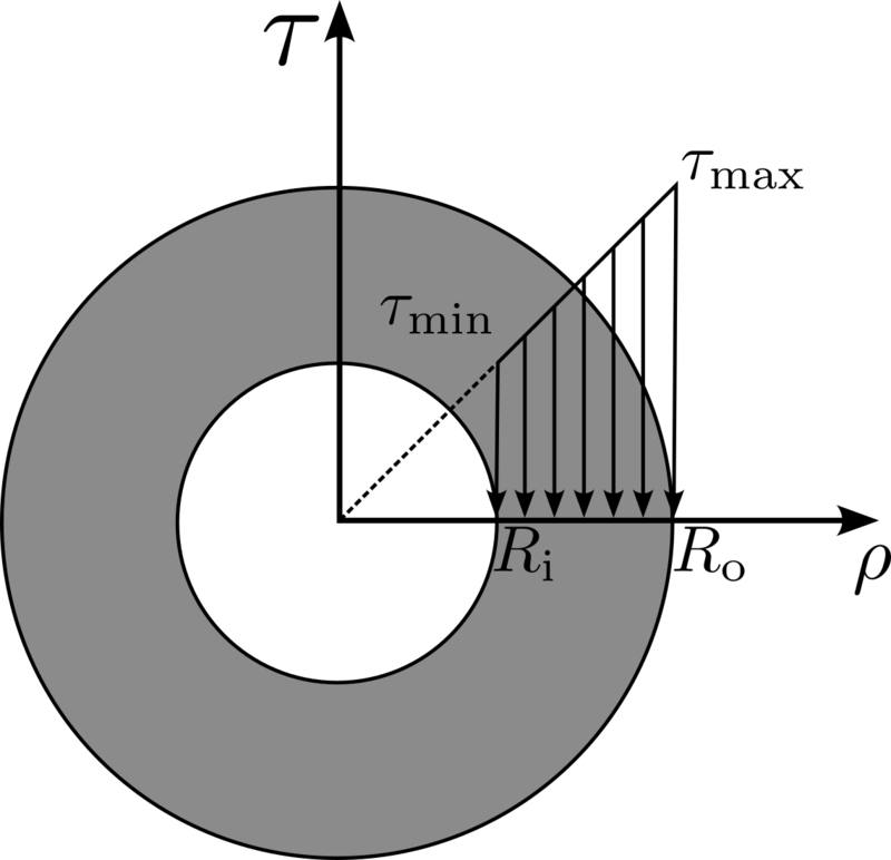
We note that this implies that under our assumptions, the shearing stress varies linearly with respect to the radial location as demonstrated in figure 15.
Figure 15: Shearing stress distribution on a hollow circular cross section. Adapted from [1].
The sum of the moments of these forces must total the applied torque:
Utilizing the relationship from equation we have
Recognizing that is the definition for the polar moment of inertia, we simplify to
Which can be rearranged to find
or to compute the shear stress at any internal radius
Having a relationship for we recall Hooke’s law for shear (equation ), make the relevant substitutions and solve for
Further recalling equation we state the following equality
which we solve for the angle of twist:
We further note that is linear with respect to the length of the shaft, so we can determine the expected rotation angle of any point on the outer surface, at any distance along the length of the shaft
2.1.4.7 Results
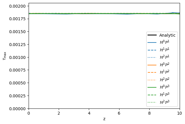
The results of the verification test are shown in the figures below. In figure 16 and figure 17 we plot the rotation angle along a line from to . We note that the bodyfit approach has some error in the coarser meshes, however they converge to the expected solution with mesh refinement, while the immersed approach is highly accurate even for the coarsest meshes. In figure 18 and figure 19 we plot the maximum shear stress along the same line, where we expect the maximum shear stress to be experienced. Again we note that the bodyfit approach has some error in the coarser meshes, however they converge to the expected solution with mesh refinement, while, once again, the immersed approach is highly accurate even for the coarsest meshes.
Figure 16: Rotation along the length of the shaft for the bodyfit meshing approach.
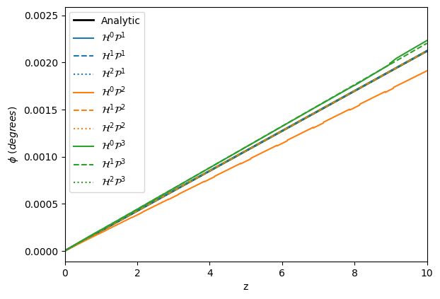
Figure 17: Rotation along the length of the shaft for the immersed rectilinear meshing approach.
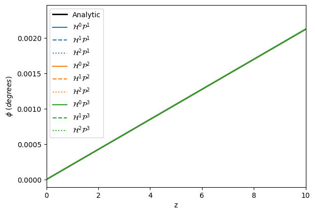
Figure 18: Maximum shear stress along the length of the shaft for the bodyfit meshing approach.
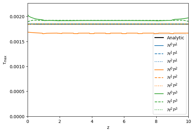
Figure 19: Maximum shear stress along the length of the shaft for the immersed rectilinear meshing approach.
2.1.5 Stresses in long pressurized pipe with butt-welded supporting trunnion pipes
2.1.5.1 Objective
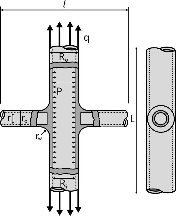
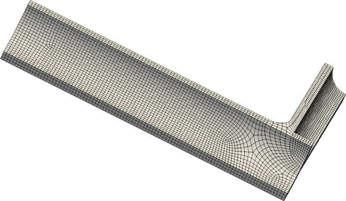
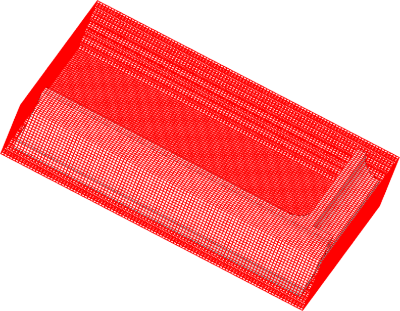
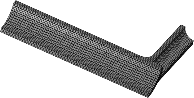
In this verification problem, the maximum von Mises stress is computed for a supported, pressurized pipe under a tension load. The pipe is supported by two trunnions that have been butt-welded to the pipe as shown in figure 20. The results are compared with the reference solution published in the NAFEMS report [5].
The Infinite plate with a hole verification problem showed that the flex method is able to accurately represent stresses in trimmed elements for a simple geometry where an exact stress field is known. In this problem, the geometry is more representative of a real-world part wherein an exact stress is not known because of the geometric complexity. In general, as the complexity of CAD parts increases, the complexity of the trimmed elements will also increase. However, it is important to keep in mind that the trimmed elements are only used to define the region in which evaluations of the background spline will be performed. The computations themselves will always be performed on the well-behaved functions of the background spline, which provides accurate results in trimmed elements. The presented results show that the flex method is able to accurately predict the maximum von Mises stress for this problem using a relatively coarse background spline.
A comparison between a conformal body-fitted approach and the fully-immersed flex approach is also shown in the results. The body-fitted approach required additional work to decompose the geometry into hex-meshable sections. The results show that both approaches produce excellent stress approximations for relatively coarse meshes. The flex approach, however, requires much less work because there is no need to decompose the geometry.
2.1.5.2 Geometry Description
2.1.5.3 External Interactions
2.1.5.4 Material Description
2.1.5.5 Method
Figure 21: The 5mm body-fitted mesh at top, followed by the untrimmed background spline and trimmed U-spline for the 5mm immersed case.
2.1.5.6 Solution Characteristics
Mesh Convergence Iteration
Mesh Size (mm)
Maximum Von Mises Stress (MPa)
Table 14: Reference solution convergence results. The mesh size column reports the mesh edge length in the area where the maximum stress occurs.
2.1.5.7 Results
Mesh scheme
Mesh size (mm)
Max. von Mises stress (MPa)
Percent difference
Body fit coarse
10
508
4.8
Body fit medium
5
516
3.4
Body fit fine
2.5
526
1.5
Immersed coarse
10
519
2.7
Immersed medium
5
530
0.7
Immersed fine
2.5
533
0.1
Table 15: Convergence results for the body-fitted and immersed simulations.
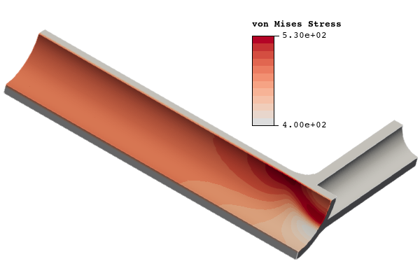
Figure 22: Comparison of immersed versus body-fitted von Mises stress and displacement for the fine mesh. The von Mises stress is shown in units of megapascals (MPa) and displacements are given in units of millimeters (mm). The minimum value for von Mises stress contours is set at 400 MPa to better show contours around the maximum value.

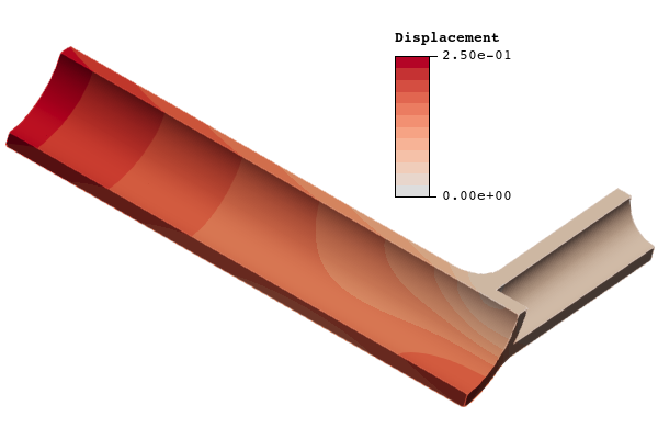

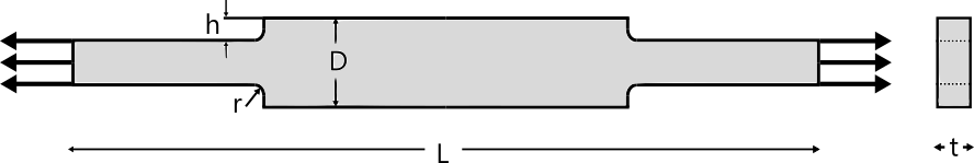
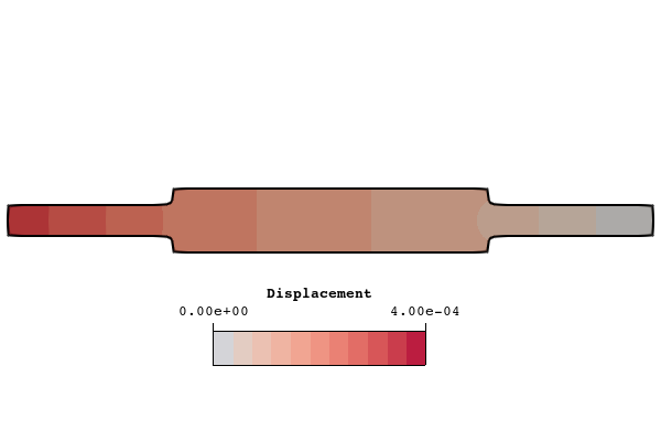
2.1.6 Stress Concentrations: filleted square shoulder of rectangular section
2.1.6.1 Objective
Predict the stress concentration factor in a member of rectangular section with a filleted square shoulder in axial tension.
2.1.6.2 Geometry Description
2.1.6.3 External Interactions
One end is fixed, and the other is given an applied pressure of .
2.1.6.4 Material Description
Mass Density
Young's Modulus
Poisson's Ratio
2.1.6.5 Method
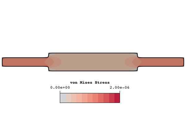
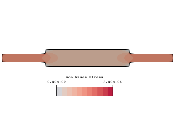
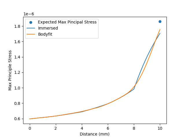
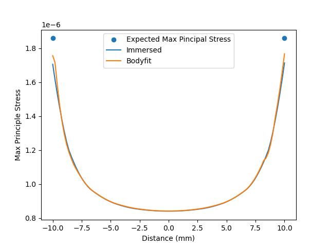
The displacements are approximated for two cases; an immersed approach and a body fit approach. In the body fit approach the volume is meshed in Coreform Cubit with a requested mesh size of 2.0. In the immersed approach the volume is immersed in a rectilinear background mesh with a mesh size of 2.0. Each case uses a quadratic spline basis to approximate displacements.
2.1.6.6 Solution Characteristics
The stress concentration factor, , is calculated using a cubic polynomial approximation:
For the cases where:
For the specific problem at hand we calculate the stress concentration factor to be . The expected maximum principal stress is .
2.1.6.7 Results
Mesh Scheme
Maximum Principal Stress
Percent Difference from Analytic Solution
BodyFit
4.9 %
Immersed Rectilinear
8.4 %

Problem Time Metric
BodyFit
Immersed rectilinear
Initialization Time
1.383e-05
2.098e-05
Linear Equation Assembly Time
0.142
0.160
NonLinear Equation Assembly Time
0.530
0.482
Solver Time
0.805
0.773
Problem Size Metric
BodyFit
Immersed rectilinear
Quadrature Points
80433
88263
Degrees of Freedom
53901
33525
2.2 Large Deformation
2.2.1 Large and small deformation of composite geometry with material interface connections and merged surfaces
2.2.1.1 Objective
The objective of this problem is to demonstrate that Coreform IGA can accurately predict small and large displacements. Additionally, it demonstrates displacement accuracy in a composite body in which the components are connected via merged geometry in one case and via material interfaces in another. Finally this problem demonstrates displacement accuracy with both linear and nonlinear material models. The problem is a simple patch test in which the displacements at the boundaries are prescribed and the displacements on the interior are easily validated against an analytical solution.
2.2.1.2 Geometry Description
2.2.1.3 External Interactions
The displacement on each boundary face is prescribed according the following function is the current time, and are the spatial coordinates. The output of this function is scaled by a parameter denoted by that varies between test cases to produce large and small displacements.
2.2.1.4 Material Description
2.2.1.5 Method
Case Number
Mesh Type
Material Model
Interface connection
Displacement Scale
Body-fit
Linear elastic
Merged
Body-fit
Neohookean
Merged
Body-fit
Neohookean
Merged
Body-fit
Neohookean
Merged
Body-fit
Neohookean
Material Interface
Body-fit
Neohookean
Material Interface
Body-fit
Neohookean
Material Interface
Immersed
Neohookean
Material Interface
In each case, the displacements are approximated with a quadratic spline basis.
For the body-fit cases, the composite body is meshed in Coreform Cubit. Each component volume is assigned a requested interval size of 1, so in the resulting mesh each component cuboid is a single hex element.
For the immersed case, the composite cube is immersed in a rectilinear background grid with a mesh size of 0.5 in each coordinate direction. Note that in the immersed case we use quadrature rule of degree 5, which is higher than the default of QP1.
For the merged geometry cases, a merge operation is performed in Coreform Cubit that merges the interface surfaces. This forces the resulting body fit mesh to be contiguous and watertight.
For the material interface cases, interface surfaces are automatically detected in Coreform Flex and a tied constraint is enforced between each pair of interface surfaces.
The displacement scale is a parameter that scales the output of the displacement boundary condition function described in the interactions section. A value of corresponds to a large displacement scenario, corresponds to a small displacement and is somewhere in between.
A probe is defined to measure the displacements at the center of the cube. Another is defined to measure displacements at the location , which is the location of maximum displacement.
2.2.1.6 Solution Characteristics
The expected displacement at any point and time can be calculated with the equation used for the prescribed boundary displacements.
2.2.1.7 Results
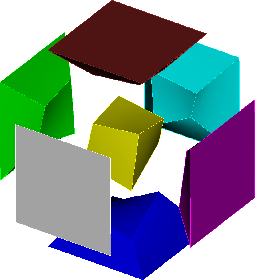
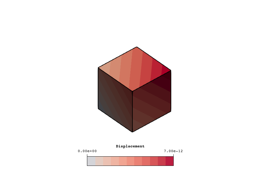
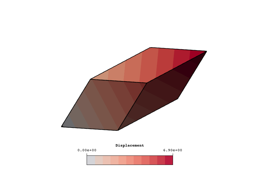
A visualization of the displacements for each displacement scale is shown in figure 28 - figure 30. The probe results and error values for each case are tabulated in table 25 - table 32.

Coordinate Direction
Center Expected Value
Center Measured Value
Center Relative Error
Max Expected Value
Max Measured Value
Max Relative Error
x
0.00 %
0.00 %
y
0.00 %
0.00 %
z
0.00 %
0.00 %
Coordinate Direction
Center Expected Value
Center Measured Value
Center Relative Error
Max Expected Value
Max Measured Value
Max Relative Error
x
0.00 %
0.00 %
y
0.00 %
0.00 %
z
0.00 %
0.00 %
Coordinate Direction
Center Expected Value
Center Measured Value
Center Relative Error
Max Expected Value
Max Measured Value
Max Relative Error
x
0.00 %
0.00 %
y
0.00 %
0.00 %
z
0.00 %
0.00 %
Coordinate Direction
Center Expected Value
Center Measured Value
Center Relative Error
Max Expected Value
Max Measured Value
Max Relative Error
x
0.00 %
0.00 %
y
0.00 %
0.00 %
z
0.00 %
0.00 %
Coordinate Direction
Center Expected Value
Center Measured Value
Center Relative Error
Max Expected Value
Max Measured Value
Max Relative Error
x
0.00 %
0.00 %
y
0.00 %
0.00 %
z
0.00 %
0.00 %
Coordinate Direction
Center Expected Value
Center Measured Value
Center Relative Error
Max Expected Value
Max Measured Value
Max Relative Error
x
0.00 %
0.00 %
y
0.00 %
0.00 %
z
0.00 %
0.00 %
Coordinate Direction
Center Expected Value
Center Measured Value
Center Relative Error
Max Expected Value
Max Measured Value
Max Relative Error
x
0.00 %
0.00 %
y
0.00 %
0.00 %
z
0.00 %
0.00 %
Coordinate Direction
Center Expected Value
Center Measured Value
Center Relative Error
Max Expected Value
Max Measured Value
Max Relative Error
x
0.03 %
0.00 %
y
0.02 %
0.00 %
z
0.02 %
0.00 %
2.2.2 Mooney-Rivlin material verification
2.2.2.1 Objective
This problem demonstrates that the results obtained when using the Mooney-Rivlin material model are consistent with analytical values derived from the underlying material formulation. The problem is setup to follow the biaxial tension test described in Cheng and Zhang [2] and uses the equations derived there to calcuated an analytical expected value for the displacment of the material.
2.2.2.2 Geometry Description
2.2.2.3 External Interactions
Face
Constraint variable
Constraint value
-X
X Displacement
-Y
Y Displacement
-Z
Z Displacement
Face
Load type
Value
+X
Surface Pressure
+Y
Surface Pressure
2.2.2.4 Material Description
Shear modulus 1
5.95522e+05
Shear modulus 2
5.03810e+04
Bulk modulus
1.0e+11
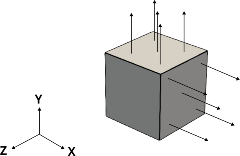
2.2.2.5 Method
The cube is meshed with a single hex element in Coreform Cubit. The boundary conditions and load conditions are defined in Coreform Flex. A probe is defined at the corner formed by the intersection of the +X, +Y and +Z faces to record the displacements in each coordinate direction. The problem is solved in Coreform IGA with the continuation timestepper, resulting in a static solution.
2.2.2.6 Solution Characteristics
As outlined in Cheng and Zhang [2], the setup of this test leads to a simplfied expression for the nominal stress in the body
where is the nominal stress, is the stretch, defined as the ratio between the deformed length and the original length, and , are the 1st and 2nd shear modulii for the material. This expression is derived from an expression of the 2nd Piola Kirchoff stress tensor as a function of the partial derivatives of the Mooney-Rivlin strain energy density. The nominal stress at our probe location is a known value uniquely determined by the applied pressure, so the above expression can be used to solve for the expected stretch and by extension the expected displacements at the probe location.
2.2.2.7 Results
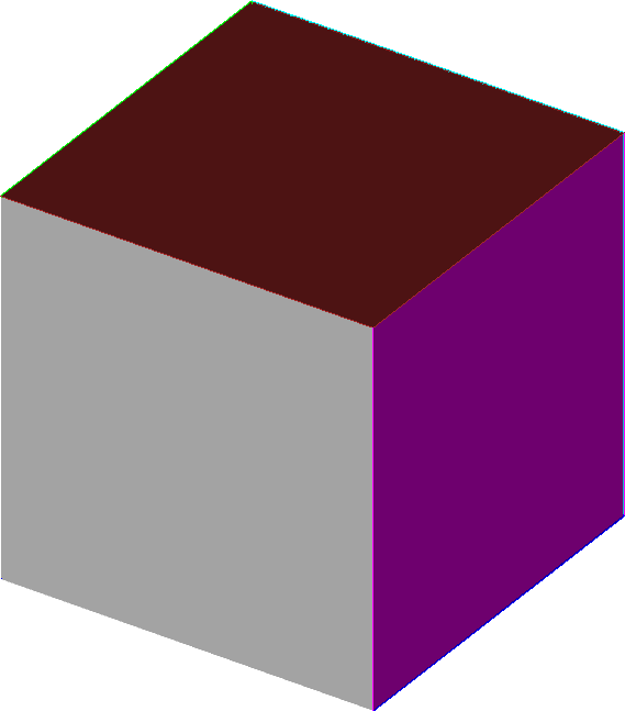
A visualization of the displacement field is shown in figure 32. The probe results and error values are tabulated in table 36.
Coordinate Direction
Expected displacement
Measured displacement
Relative error
x
0.02 %
y
0.02 %
z
0.00 %
2.3 Incompressible Elasticity
2.3.1 Neo-Hookean cylindrical pressure vessel
2.3.1.1 Objective
The main purpose of this test is to demonstrate the accuracy of the neo-Hookean hyperelastic material model in a finite-strain problem with a known non-trivial analytical solution. In particular, we solve the problem of a plane-strain section of a cylinder subjected to internal pressure. This problem was used to verify an academic implementation in Section 3.2 of [2]. A secondary purpose of this test is to demonstrate the effectiveness of higher-order immersed analysis in a situation where classical low-order finite element analysis would be affected by severe "locking" due to a large bulk modulus.
2.3.1.2 Geometry Description
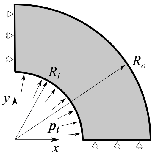
2.3.1.3 External Interactions
To model a full cylinder subject to plane-strain kinematics, we apply the symmetry boundary conditions shown in figure 33, and additional symmetry boundary conditions on the faces. The inner surface of the cylinder is subject to a pressure follower load of magnitude . This is treated as given data in the problem setup, but chosen based on an analytical solution to result in a known radial displacement of the inner surface, via equation . The outer surface of the cylinder is traction-free. The symmetry boundary conditions use a dimensionless penalty scale factor of 1000 to perform a controlled study on the accuracy of the constitutive model and potential for locking in high-order splines.
2.3.1.4 Material Description
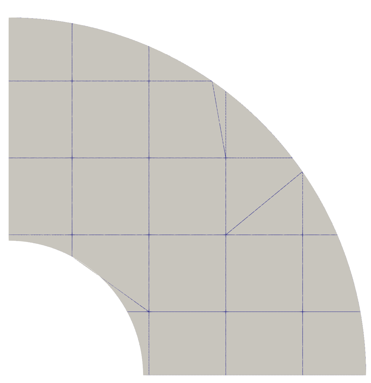
2.3.1.5 Method
2.3.1.6 Solution Characteristics
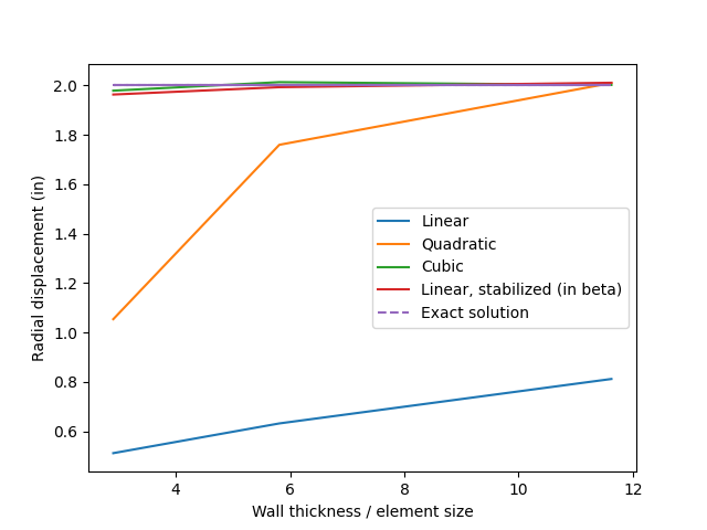
An analytical solution is available from the literature [2] for the fully-incompressible case, which we are approximating via . For the mesh sizes considered here, the error due to this approximate incompressibility is small relative to the approximation error inherent in using polynomial splines to approximate a transcendental exact solution. The exact solution is most conveniently parameterized in closed form by considering a target radial displacement of the inner surface, , and then calculating the corresponding pressure as where This solution is valid for arbitrarily-large deformations, and we select for calculating the results presented here, corresponding to an applied follower pressure of psi.
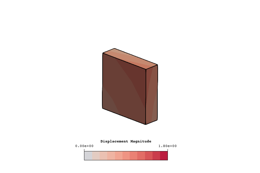
2.3.1.7 Results
2.4 Plasticity
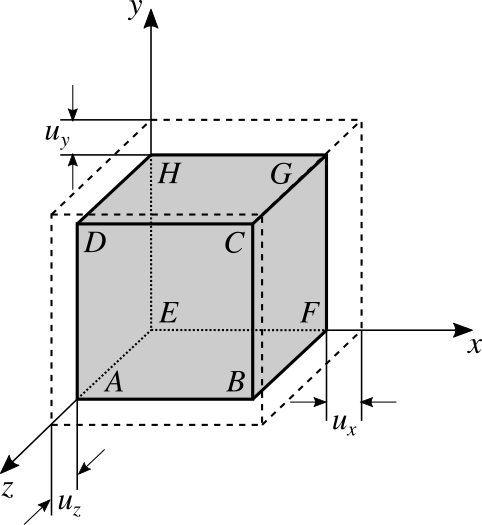
2.4.1 J2 plasticity: 3D unit cube with isotropic hardening
2.4.1.1 Objective
This verification problem benchmarks static elasto-plastic deformation in a single 3D element with isotropic hardening against results published by NAFEMS [3]. It demonstrates accurate stress predictions for a nonlinear material with higher order spline basis functions.
2.4.1.2 Geometry Description
2.4.1.3 External Interactions
Boundary conditions prescribing displacement values are created for each face of the cube. The type of boundary condition for each face is tabulated in table 38. The prescribed displacement values vary depending on the stage of the simulation and are explained in table table 40.
Location
Constraint
Face AEHD
Translation along x-axis fixed
Face ABFE
Translation along y-axis fixed
Face EFGH
Translation along z-axis fixed
Face BCGF
prescribed
Face CDHG
prescribed
Face ABCD
prescribed
Table 38: Boundary conditions for the 3D elastoplasticity verification problem.
2.4.1.4 Material Description
Property
Value
Mass Density
0
Young's Modulus
2.5e5
Poisson's Ratio
0.25
Yield Stress
5.0
Isotropic Hardening Modulus
6.25e4
2.4.1.5 Method
In this test, the cube is meshed with a single 3d element and displacements are calculated using a cubic spline basis. The cube is loaded in tension along a combination of its two axes, in plane strain, before being returned to zero displacement boundary conditions. The loading pattern is shown in table 40.
Step
1
R
0.0
0.0
2
2R
0.0
0.0
3
2R
R
0.0
4
2R
2R
0.0
5
2R
2R
R
6
2R
2R
2R
7
R
2R
2R
8
0.0
2R
2R
9
0.0
R
2R
10
0.0
0.0
2R
11
0.0
0.0
R
12
0.0
0.0
0.0
Table 40: Loading conditions for the 3D elastoplasticity verification problem.
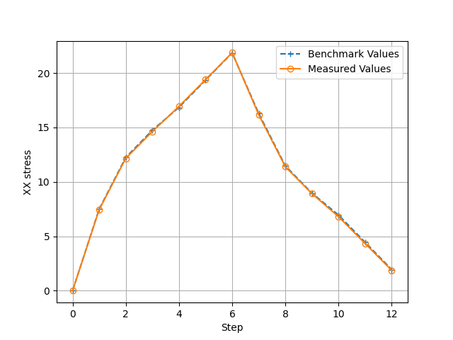
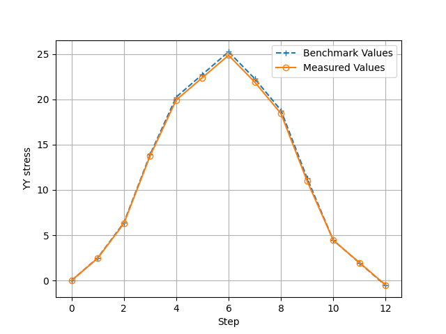
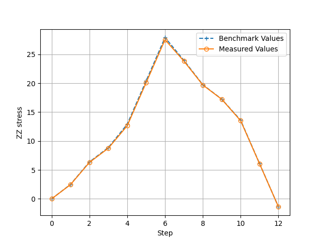
2.4.1.6 Results
Stress results are plotted alongside benchmark values in figure 37 - figure 40. The benchmark values are from results published in the reference text [3].

2.5 Mechanical Contact
2.5.1 Interference fit of two pipes
2.5.1.1 Objective
Interference fits are a common technique used to join parts through friction by requiring deformation in order to fit the parts together and inducing initial stress and contact forces. In analysis, the parts are initially undeformed and they overlap at the interface. A robust contact algorithm is required to resolve the overlap and produce an accurate initial displacement.
Additionally, it is very common for modeling errors to create unintentional small initial penetrations that can lead to erroneous behavior in an analysis if left unresolved. Manually resolving initial penetrations can be significantly time consuming, so it is important that a contact algorithm is able to automatically detect and resolve initial penetrations.
This current problem demonstrates the ability of Coreform IGA to accurately resolve initial penetrations. The geometry, boundary conditions and loading of this problem create a small deformation, plane strain axi-symmetric setting that allows for a relatively simple closed form analytical solution against which the analysis results can be validated.
2.5.1.2 Geometry Description
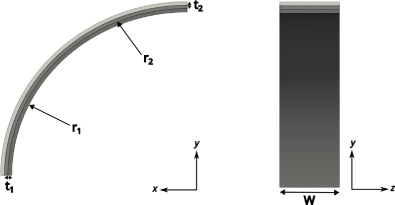
2.5.1.3 External Interactions
Symmetry boundary conditions are enforced in the and directions. Specifically, the faces of each part are constrained to have no displacement in the direction, and the faces are constrained to have no displacement in the driction. Additionally, the and faces of both parts are constrained to have no displacement in the direction to restrict rigid body translation.
The inner surface of the larger part and the outer surface of the smaller part are included in a surface to surface contact definition.
We use a dimensionless penalty scaling factor of for all displacement boundary conditions to ensure accuracy of the applied constraints. This high penalty scaling factor is used for this problem because we are comparing the computed solution to a known reference solution. In most practical applications the default penalty scaling values would produce a solution this is good enough.
2.5.1.4 Material Description
2.5.1.5 Method
We approximate the displacements in each cylinder using quadratic trimmed splines defined on a background mesh with element size of 0.03. We use a implicit statics time stepper based on numerical continuation to solve the nonlinear problem in multiple steps.
The resolution of interference fit relies on the regular contact algorithm to find the equilibrium configuration by removing the initial penetration under the quasi-static condition. See the theory manual for details. For this problem we use an initial activate distance of 0.04 and a ramp time interval of .
We define probes to measure the displacement in each coordinate direction at the points and . These point correspond to locations halfway long the cylinder width, at the outer radius of the larger cylinder and the inner radius of the smaller cylinder. The displacement at these points is compared to an analytical solution. We define an additional probe that measures the contact force that develops due to the contact defined between the two cylinder parts. The value measured is compared to an analytical solution.
2.5.1.6 Solution Characteristics
The analytical solution is derived in the plane-strain axisymmetric setting under small deformation. In the plane-strain axisymmetry, only the radial displacement component, , is nonzero. For strain, likewise, only the radial, , and circumferential strain, , are nonzero, where denotes the radial position. In the absence of Poisson’s ratio and a body force, the equilibrium in a single body is represented by the following equation:
Note that it is not necessary to have a Dirichlet boundary condition even for a static problem, as the plane-strain axisymmetric condition provides enough constraints.
The solution for the inner pipe, , and the one for the outer pipe, , that satisfy the above equation are
with the unknown constants , , and .
Next, we apply the traction boundary and interface conditions. where are defined in table 43, denotes the contact pressure, and denotes the displacement at the inner surface of the outer pipe, i.e. the interface displacement of the outer pipe.
2.5.1.7 Results
Value
Measured value
Analytical solution
Relative error
Inner pipe displacement
2.7 %
Outer pipe displacement
1.1 %
Reaction force X
1.8 %
Reaction force Y
1.8 %
Figure 42: X displacement field after interference resolution